MIME KNN: Improve KNN Classifier Performance Include Classification Accuracy and Time Consumption

1

2018 International Conference on Computer Science and Software Engineering (CSSE 2018) ISBN: 978-1-60595-555-1

MIME-KNN: Improve KNN Classifier

Performance Include Classification

Accuracy and Time Consumption

Taizhang Shang, Xiang Xia and Jun Zheng

ABSTRACT

The K Nearest Neighbor (KNN) classifier has been widely used in the applications of data mining and machine learning, because of its simple implementation and distinguished performance. However, because the distance between all training samples and test samples have to be calculated, when there are too many samples or samples have huge features dimensionality, the time complexity and space complexity are high. The paper proposes a KNN algorithm with the minimum intra-class distance and the maximum extra-class distance (MIME-KNN). By finding a transformation matrix, the algorithm minimizes the intra-class distance and maximizes the distance between classes, which can improve the classification performance of traditional KNN algorithm. At the same time, the algorithm will also reduce the dimensionality of the samples to achieve the purpose of reducing time and space complexity. Experimental results show that the MIME-KNN work well in practical.

INTRODUCTION

Classification is one of the most important research topics in pattern recognition and data mining domain [1,2]. Over the past decades, many classification algorithms have been proposed [3-6], K Nearest Neighbors

Taizhang Shang1,2*, Xiang Xia1,2 and Jun Zheng1,2

1

School of Automation, Huazhong University of Science and Technology (HUST), Wuhan, China

2

Key Laboratory of Image Information Processing and Intelligent Control, Ministry of Education, Wuhan 430074, China

algorithm is one of the most important classification algorithms, and has been regarded as one of the top 10 data-mining algorithms [7].

The K-nearest neighbor classification algorithm is simple and effective, and widely used in practical. The core idea of the KNN algorithm is that in a space with an unknown sample, the data class of the sample can be determined based on the data classes of the k nearest samples from this sample. It has many advantages, such as the theory of the algorithm is easy to understand, and the algorithm is very simple to implement. However, the algorithm still has many places for further research and promotion. the similarity measurement between two data points and the selection of the k value [8]. Many methods have been proposed to address these two issues [9,10,11,12]. In addition to these two issues, KNN has other areas that can be further optimized. This article focuses on reducing the time complexity of classification and improve the recognition performance, and proposed minimize intra-class distance and the maximize out-class distance KNN algorithm (MIME-KNN).

The purpose of MIME-KNN is to map the original sample to the low-dimensional space, and to minimize the intra-class distance, and to maximize the extra-class distance of the samples in the low-dimensional space. In this way, it is possible to compress the same class of samples as much as possible within a small range, so that the KNN algorithm is more robust to K, and reducing dimensionality can reduce the time and space complexity. So the key problem of MIME-KNN is how to find the transpose matrix to map the original sample to low-dimensional space.

In this paper, we use several datasets from UCI repository of machine learning databases. For evaluation, several experiments have been carried out on these data sets. Results show that MIME-KNN can not only reduce the time complexity of the classical KNN by reducing the data set dimension, but also improve the classification performance of the classical KNN algorithm. In addition, we have added noise to the dataset and analyzed the noise immunity of the improved KNN algorithm.

The contributions of this paper can be summarized as follows:

(1) We theoretically prove the effectiveness of the algorithm.

(2) We experimentally demonstrate the advantages of the algorithm over the classical KNN algorithm.

THE MIME-KNN ALGORITHM

Classical KNN Algorithm

The KNN algorithm is a classification algorithm and can also be used as a regression algorithm. Here we only discuss the use as a classification algorithm. KNN is a case-based learning method, which keeps all the training data for classification, and does not require training before classifying test samples. KNN

algorithm obtains the approximate solution Cˆ of the classification function C which works as follows: Given a distance function dist : , the set

pk train

N ⊆C

denotes the k nearest neighbors of p in training set Ctrain. The class ˆ

pk

C

assigned to point p is the majority class within this set of k nearest neighbors

pk

N

. What the MIME-KNN algorithm does is to preprocess the data before the classical KNN algorithm, specifically to compress the same type of data into a small range, increase the distance between different classes, and reduce the dimensionality of data to Reduce Time and Space Consumption of KNN Algorithm at the same time.

MIME-KNN Algorithm

The MIME step divides the training dataset into two parts, the class TC and the other class OC (every class will be selected as TC in turn, and the others will be OC). The algorithmic procedure is formally stated below:

1. Calculate the center vectors for each category: Calculate the mean vector of each feature of all the sample points in the same class, and the mean vector is used as the center vector of the class.

2. Choose the point weight function: we provide two functions here.

The sample points of the OC near the TC center and the sample points of the TC far from the TC center, will have more effect on minimizing the intra-class distance, and maximizing the extra-class distance of the samples in the low-dimensional space. So algorithm should give more focus on these sample points. Motivated by this, the point weight function is supposed like following:

2

1

i tc

x meanvec i

q e τ

 − 

−_ −_

 

1

1

j tc

x meanvec j

p e τ

 ₋ 

 −

 

 

= (2)

Where qi represents the weight for sample i of the OC, xi represents sample i of OC, meanvectc represents the center vector of TC, τ₂ represents the average distance of all the sample points of OC from the center point of TC. p_j represents the weight for sample j of the TC, x_j represents sample j of TC, τ₁ represents the average distance of all the sample points of TC from the center point of TC.

Simple as following:

1

i j

q =p = (3)

It means all the sample points of OC and TC are weighted the same, regardless of the distance from the TC center.

3. Mapping: Calculate the eigenvectors and eigenvalues of classical eigenvector problems:

1

( ( ) ( ) ( ) ( ) )

tc oc tc

T T

oc tc oc tc tc tc tc tc

C C C

X meanvec Q X meanvec X meanvec P X meanvec a λa

−

− − − − − =

∑∑ ∑ (4)

Where Xocrepresents the matrix of all the samples in the OC. Let a a0, ...1 am−1

be the eigenvectors corresponding to λ₀>λ₁>...>λ_m−₁ (λ λ λ0, ...1 d−1 are the solution of λ in Equation (4) ), and the transformation matrix A is composed of the first d eigenvectors ( a a0, 1...ad−1

) of a, d is the dimensionality of dataset after dimensionality reduction. Then use the transformation matrix A to map the samples in original space to a d-dimensional space as the following formula.

0 1 1

, ( , ,..., )

T

i d

i

y =A x A= a a a −

(5) Where A is the transformation matrix, xi

is the sample point in original space, and yi

is the corresponding point in the low-dimensional space.

At this point, all the training data xi

has been mapped to yi

in low-dimensional space, and the purpose of minimize the intra-class distance, and maximize the extra-class distance of the samples in the low-dimensional space has been achieved. For a new test sample xt

, we only need to use the transformation matrix A to map the test sample xt

to y_t

in low-dimensional

space: T t t

y =A x

. Then y_i

will be the train samples and y_t

will be the test sample for KNN step.

Justification

The purpose of the MIME step is minimizing the intra-class distance, and maximizing the extra-class distance of the samples in low-dimensional space. Give the original dataset x x₁,₂...x_m∈Rn

these original sample points to a low-dimensional space with the formula:

T i i

y =A x

. So the key problem is how to find the transform matrix A. Here we have a reasonable criterion for choosing a good map is to maximize the following objective function under appropriate constraints:

2 2

1 1 1

max( (( ) ) (( ) ))

tc oc k _i tc k _j

tc i tc j

oc tc

C C i C i

y meanvec q y meanvec p

− = =

− − −

∑∑∑

∑∑

Where yi_oc

is i-th sample point of OC, y_tcj

is j-th sample point of TC. qi represents the weight for sample i of the OC, and p_j represents the weight for sample j of the TC. qi is chosen based on the distance of sample i of the OC from the center of TC, the sample which is more close to the center of TC need more attention. p_j is chosen based on the distance of sample j of the TC from the center of TC, the sample which is farther from the center of TC need more attention. So the optimization of the objective function is to try to make sample points of different class away from each other, and Sample points of the same class are clustered in a smaller range. Two qi and pj function have been

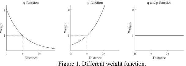
proposed in last section. The relationship between the distance of sample i from the center of TC and the weight of sample i is shown in Figure 1 below.

In Figure 1, The first plot shows the relationship between distance of samples in OC from the center of TC and the weight qi of responding samples with

formula (1). The second plot shows the relationship between distance of samples in TC from the center of TC and the weight p_jof responding samples with formula (2). The third plot shows the same relationship in formula (3). τ

represents the average distance of all the sample points of OC from the center point of TC in first plot and the average distance of all the sample points of TC from the center point of TC in second plot. The vertical axis represents the weight of the sample point of OC in first plot and weight of the sample point of TC in the second plot, and the horizontal axis represents the distance from the TC center of the sample point in OC in first plot and the distance from the TC center of the sample points in TC in second plot.

Figure 1. Different weight function.

Suppose a

is a unit transformation vector, that is, T T i i

y=a x =x a

2 2

1 1 1

1 1 1

(( ) ) (( ) )

( ) ( ) ( ) ( )

(( ' ) )

tc oc k tc k

i j

tc i tc j

oc tc

C C i C j

tc oc k _{i i} tc k _{j j}

T T

tc i tc tc j tc

oc oc tc tc

C C i C j

i _{T T}

oc _tc

y meanvec q y meanvec p

y meanvec q y meanvec y meanvec p y meanvec

x meanvec a

− = = − = = − − − = − − − − − = − ∑∑∑ ∑∑ ∑∑∑ ∑∑

1 1 1

1 1

( ' ) (( ' ) ) ( ' )

( ' ) ( ' ) ( ' ) ( ' )

tc oc k tc k

i _T j _{T T} j _T

oc tc tc

i tc tc i tc

C C i C j

tc oc k _{i i j j}

T T T T

oc tc i oc tc tc tc i tc tc

C C i

q x meanvec a x meanvec a p x meanvec a

a x meanvec q x meanvec a a x meanvec p x meanvec a

− = = − = − − − − = − − − − − ∑∑∑ ∑∑ ∑∑∑ 1 1 1 ( ( ' ) ( ' ) ) ( ( ' ) ( ' ) ) ( ( ' ( ' ) ( ' ) ( ' ) ) tc k C j

tc oc tc

T T T T

oc tc oc tc tc tc tc tc

C C C

tc oc tc

T T T

oc tc oc tc tc tc tc tc

C C C

a X meanvec Q X meanvec a a X meanvec P X meanvec a

a X meanvec Q X meanvec X meanvec P X meanvec a

= − − = − − − − − = − − − − − ∑∑ ∑∑ ∑ ∑∑ ∑

Where Q is a diagonal matrix composed of q_i, P is the diagonal matrix composed of p_j, meanvec_tcis the center of class after dimension reduction, and

'_tc

meanvec is the center of the class before dimension reduction. Then the

purpose of the algorithm is converted to the maximum of the upper expression, suppose the maximum value of the objective is λ

1

( ( ' ) ( ' ) ( ' ) ( ' ) )

tc oc tc

T T T

oc tc oc tc tc tc tc tc

C C C

a X meanvec Q X meanvec X meanvec P X meanvec a λ

−

− − − − − =

∑∑ ∑

For a

is a unit transformation vector, T 1

a × =a

. The right side of the formula multiplied by a, we get this:

1

( ( ' ) ( ' ) ( ' ) ( ' ) )

tc oc tc

T T

oc tc oc tc tc tc tc tc

C C C

X meanvec Q X meanvec X meanvec P X meanvec a λa

−

− − − − − =

∑∑

∑

1

( ' ) ( ' ) ( ' ) ( ' )

tc oc tc

T T

oc tc oc tc tc tc tc tc

C C C

X meanvec Q X meanvec X meanvec P X meanvec

−

− − − − −

∑∑

∑

is a symmetric matrix. In this way, the target problem is transformed into the classic eigenvalue and eigenvector problem. This can be solved easily. After getting all the eigenvalues and eigenvectors, we sort all the eigenvalues by descending order λ₀>λ₁>...>λm−₁ and take the first d corresponding eigenvectors (a a0, 1...ad−1

) to form transformation matrix A. Then we can use the transformation matrix A to map the samples in original space to a d-dimensional space as the following formula.

0 1 1

, ( , ,..., )

T

i d

i

y =A x A= a a a −

Where A is the transformation matrix, xi

is the sample point in original space, and y_i

This section is the Justification of MIME step. It will be classical KNN step after MIME step in the MIME-KNN algorithm. The classical KNN algorithm has been described in section 2.1, it is easy to understand.

EXPERIMENTS AND RESULTS

In order to verify the effectiveness of MIME-KNN, MIME-KNN has been compared with classical KNN algorithm on 4 datasets: TTC-3600: Benchmark dataset for Turkish text categorization Data Set, Molecular Biology (Splice-junction Gene Sequences) Data Set, Glass Identification Data Set and Connectionist Bench (Sonar, Mines vs. Rocks) Data Set. They are all get from UCI repository of the machine learning databases [13]. The experiment consists of three parts, the comparison of accuracy, the robustness of the algorithm to noise and the comparison of recognition time. In all experiments, the similarity evaluation criteria used by MIME-KNN and KNN are Euclidean distances, and the K value is selected by cross-validation.

Comparison of MIME-KNN and KNN

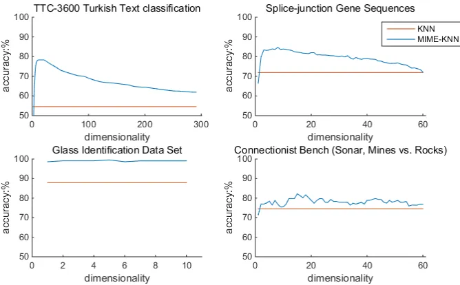
In order to highlight the improvement of the recognition accuracy of MIME-KNN compared to the classical MIME-KNN algorithm, we compared the accuracy of MIME-KNN and classical KNN algorithms on these data sets. In the experiment, 5 fold cross-validation method is used [14], randomly select 80% of the data for training, the remaining 20% of the data for testing, repeat the experiment 5 times. And then take the average accuracy of the result in cross-validation as the final classification accuracy. And the comparison result is shown in Figure 2.

From Figure 2 we can clearly see that the MIME-KNN algorithm can reduce the data set to a very low dimension while improving the recognition rate of the classical KNN algorithm. And in the MIME-KNN algorithm, the highest recognition rate tends to occur in the lower dimension. This can ensure high classification accuracy and reducing the time complexity and reducing space complexity in the KNN step, these three advantages occur simultaneously.

Figure 2. The classification accuracy comparison of MIME-KNN and KNN on four public datasets from UCI repository of the machine learning databases.

TABLE I. FEATURE DIMENSION, CLASSIFICATION ACCURACY AND TIME CONSUMPTION IN KNN AND MIME-KNN.

TTC-3600 Gene

Sequences Glass

Connectionist Bench

KN N

Feature

dimension 3028 60 10 60

Classification

Accuracy(%) 54.5833 71.8962 87.8918 74.5015

time consumption for

1 sample(s)

9.5985e-3 1.4531e-3

2.8206e-4 2.6855e-4

MI ME-KNN

Feature

dimension 11 8 5 12

Classification

Accuracy(%) 77.8889 84.6274 99.5455 82.2030

time consumption for

1 sample(s)

7.4443e-05 6.0898e-4

3.1493e-4 3.1409e-4

decreased by two orders of magnitude. In Glass Identification Data Set, the accuracy of classification increased by 12% and time consumption increased a little. In high-dimensional data sets, the effect of MIME-KNN on the reduction of time consumption is very obvious. However, in low-dimensional datasets, MIME-KNN will increase in time consumption, but it will only increase slightly within the same order of magnitude, and this will increase the accuracy of the classification, which is worthwhile.

Robustness of MIME-KNN to Noise

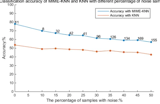
In the experiment of analyzing the robustness of MIME-KNN to noise, the data set we use is TTC-3600: Benchmark dataset for Turkish text categorization Data Set. To illustrate the robustness of the proposed feature extraction algorithm, we add different numbers of noise samples to the data and compare the classification performance using MIME-KNN and classical KNN. The percentage of noise samples vary from 10% to 50%. the result is shown in Figure 3.

In Figure 3, the blue curves represent the best classification accuracy, which MIME-KNN obtained on different percentage of noise samples. The upper number represents the number of dimensions when the highest recognition rate is obtained. The red curves represent the classification accuracy that KNN obtained on different percentage of noise samples. It can be seen that the best classification accuracy MIME-KNN obtained are always higher than the classification accuracy KNN obtained on different percentage of noise samples. And even the best classification accuracy of MIME-KNN with 50% noise data is still higher than that of KNN with no noise data.

CONCLUSIONS

In this paper, a new KNN optimization algorithm MIME-KNN is presented. The purpose of MIME-KNN is to map the original sample to the low-dimensional space, and to minimize the intra-class distance, and to maximize the extra-class distance of the samples in the low-dimensional space. By this method, we improve the classification accuracy of the KNN algorithm and reduce the time complexity and space complexity. We theoretically prove the effectiveness of the algorithm and experimentally demonstrate the advantages of the algorithm over the classical KNN algorithm. The experiment result shows that MIME-KNN can effectively improve the classification accuracy and reduce the time complexity. Also, the robustness of MIME-KNN to noise is illustrated.

ACKNOWLEDGEMENTS

This work was financially supported in part by Cryptography Theoretical Research of National Cryptography Development Fund (Grant No. MMJJ20170109), in part by Independent Innovation Fund of Huazhong University of Science and Technology (Grant No. 2016YXMS067).

REFERENCES

1. Bijalwan V, Kumar V, Kumari P, & Pascual J (2014). KNN based machine learning approach for text and document mining. International Journal of Database Theory and Application, 7(1), 61-70.

2. Deng Z, Zhu X, Cheng D, Zong M, & Zhang S (2016). Efficient kNN classification algorithm for big data. Neurocomputing, 195, 143-148.

3. Rish I (2001, August). An empirical study of the naive Bayes classifier. In IJCAI 2001 workshop on empirical methods in artificial intelligence (Vol. 3, No. 22, pp. 41-46). IBM. 4. Safavian S. R, & Landgrebe D (1991). A survey of decision tree classifier

methodology. IEEE transactions on systems, man, and cybernetics, 21(3), 660-674.

5. Evelyn Fix and Joseph L Hodges Jr. 1951. Discriminatory analysis-nonparametric discrimination: consistency properties. Technical Report. California Univ Berkeley.

6. Suthaharan S (2016). Support vector machine. In Machine learning models and algorithms for big data classification (pp. 207-235). Springer, Boston, MA.

7. Xindong Wu, Vipin Kumar, J. Ross Quinlan, Joydeep Ghosh, Qiang Yang, Hiroshi Motoda, Geoffrey J. McLachlan, Angus Ng, Bing Liu, S. Yu Philip, and others. 2008. Top 10 algorithms in data mining. Knowledge and information systems. 14, 1 (2008), 1–37.

8. Zhang S (2010). KNN-CF Approach: Incorporating Certainty Factor to kNN Classification. IEEE Intelligent Informatics Bulletin, 11(1), 24-33.

9. Qin Y, Zhang S, Zhu X, Zhang J, & Zhang C (2007). Semi-parametric optimization for missing data imputation. Applied Intelligence, 27(1), 79-88.

11. Bhattacharya G, Ghosh K, & Chowdhury A. S (2012). An affinity-based new local distance function and similarity measure for kNN algorithm. Pattern Recognition Letters, 33(3), 356-363.

12. Zhang S, Li X, Zong M, Zhu X, & Cheng D (2017). Learning k for knn classification. ACM Transactions on Intelligent Systems and Technology (TIST), 8(3), 43.

13. Blake C L. UCI repository of machine learning databases[J]. http://www. ics. uci. edu/~ mlearn/MLRepository. html, 1998.