R E S E A R C H
Open Access
A quasi-boundary value regularization
method for identifying an unknown source in
the Poisson equation
Fan Yang
*, Miao Zhang and Xiao-Xiao Li
*Correspondence:
[email protected] School of Science, Lanzhou University of Technology, Lanzhou, Gansu 730050, People’s Republic of China
Abstract
In this paper, we consider the problem for identifying the unknown source in the Poisson equation in a half unbounded domain. A conditional stability result is given and a quasi-boundary value regularization method is presented to deal with this problem. For the regularization solution, the Hölder type stability estimate between the regularization solution and the exact solution is given. Numerical results are presented to illustrate the accuracy and efficiency of this method.
MSC: 35R25; 47A52; 35R30
Keywords: ill-posed problem; unknown source; conditional stability; quasi-boundary value; Poisson equation
1 Introduction
Inverse source problems arise in many branches of science and engineering,e.g.heat con-duction, crack identification, electromagnetic theory, geophysical prospecting, and pol-lutant detection. For the heat source identification, there have been a large number of research results for different forms of heat source [–]. To the author’s knowledge, there were few papers for identifying an unknown source in the Poisson equation using the reg-ularization method. In [], the authors identified the unknown point source with the logarithmic potential. In [], the author identified the unknown point source using the projective method. In [], the authors identified the unknown point source using the Green’s function. In [, ], the authors identified the unknown source dependent only on one variable using the dual reciprocity method. In [], the authors identified the un-known source dependent only on one variable using the method of fundamental solution. But by the regularization method, there are a few papers with strict theoretical analysis on identifying the unknown source.
In this paper, we consider the following inverse problem: to find a pair of functions (u(x,y),f(x)) which satisfy
⎧ ⎪ ⎪ ⎪ ⎪ ⎪ ⎨ ⎪ ⎪ ⎪ ⎪ ⎪ ⎩
–uxx–uyy=f(x), –∞<x<∞,y> ,
u(x, ) = , –∞<x<∞, u(x,y)|y→∞ bounded, –∞<x<∞,
u(x, ) =g(x), –∞<x<∞,
(.)
wheref(x) is the unknown source depending only on one spatial variable andu(x, ) =g(x) is the supplementary condition. In applications, input datag(x) can only be measured, there will be measured data functiongδ(x) which is merely inL(R), and it satisfies
g–gδL(R)≤δ, (.)
where the constantδ> represents a noise level of input data.
The problem (.) is ill-posed,i.e., the solution (if it exists) does not depend continuously on the data. One way to solve an ill-posed problem is by perturbing it into a well-posed one. Many perturbing techniques have been proposed, including a biharmonic regular-ization developed by Lattés and Lions in [], a pseudo-parabolic regularregular-ization proposed by Showalter and Ting in [], a stabilized quasi-reversibility proposed by Miller in [], the method of quasi-reversibility proposed by Mel’nikova in [], a hyperbolic regulariza-tion proposed by Ames and Cobb in [], the Gajewski and Zacharias quasi-reversibility proposed by Huang and Zheng in [], a quasi-boundary value method by Denche and Bessila in [], and an optimal regularization proposed by Boussetila and Rebbani in []. It appears that Showalter in [] was the first who used the quasi-boundary value regular-ization method to consider the backward heat conduction problem. In [], the authors used the quasi-boundary-value method to consider the Cauchy problem for elliptic equa-tions with nonhomogeneous Neumann data. In this paper, we use the quasi-boundary value regularization method to identify the unknown source for the Poisson equation.
The outline of the paper is as follows. Section gives an analysis on the ill-posedness of this inverse problem and some auxiliary results. Section gives a regularization solu-tion and error estimasolu-tion. Secsolu-tion gives some examples to illustrate the accuracy and efficiency of this method. Section puts an end to this paper with a brief conclusion.
2 Ill-posedness of the problem and some auxiliary results
The ill-posedness can be seen by solving the problem in the frequency domain. Let
ˆ
f(ξ) :=√ π
∞
–∞
e–iξxf(x)dx (.)
be the Fourier transform of the functionf(x).
The problem (.) can be formulated in frequency space as follows:
⎧ ⎪ ⎪ ⎪ ⎪ ⎪ ⎨ ⎪ ⎪ ⎪ ⎪ ⎪ ⎩
ξu(ˆ ξ,y) –uˆ
yy(ξ,y) =fˆ(ξ), ξ∈R,y> , ˆ
u(ξ, ) = , ξ∈R,
ˆ
u(ξ,y)|y→∞ bounded, ξ∈R,
ˆ
u(ξ, ) =g(ξ), ξ∈R.
(.)
The solution of the problem (.) is given by
ˆ
f(ξ) = ξ
–e–|ξ|g(ˆ ξ). (.)
So
f(x) =√ π
∞
–∞e
iξx ξ
The unbounded function –ξe–|ξ| in (.) or (.) can be seen as an amplification factor
ofg(ˆξ) whenξ→ ∞. Therefore when we consider our problem inL(R), the exact data functiong(ˆ ξ) must decay rapidly asξ → ∞. But in the applications, the input datag(x) can only be measured and never be exact. We assume the measured data functiongδ(x)∈
L(R). Thus if we try to obtain the unknown sourcef(x), high frequency components in the error are magnified and can destroy the solution. So it is impossible to solve the problem (.) by using the classical method. In the following section, we will use a quasi-boundary value regularization method to deal with the ill-posed problem. Before doing that, we impose ana prioribound on the input datai.e.,
f(·)Hp≤E, p> , (.)
whereE> is a constant, · Hpdenotes the norm in Sobolev spaceHp(R) defined by
f(·)Hp:=
∞
–∞
fˆ(ξ) +ξpdξ
. (.)
Now we give some lemmas which are very useful for our main conclusion.
Lemma . If x> ,we have the following inequality:
–e–x ≤
e
e– . (.)
Lemma . For <β< ,the following inequality hold:
sup
ξ∈R
βξβ+ –ξ e–|ξ|
+ξ–
p
≤maxβp,β. (.)
Proof Let
A(ξ) := β ξ
βξ+ –e–|ξ|
+ξ–
p
. (.)
The proof of (.) is separated into three cases. Case .|ξ| ≥ξ=β; we get
A(ξ)≤ +ξ–
p
≤ |ξ|–p≤ξ–p
=βp. (.)
Case . <|ξ|<ξ; we obtain
A(ξ)≤ β ξ–p
–e–|ξ| ≤β
ξ–p. (.)
If <p≤, the above inequality becomes
Ifp> , we get
A(ξ)≤βξ–p≤β. (.)
Case .|ξ| ≤; we get
A(ξ)≤ β ξ
–e–|ξ| ≤β
e e– ≤β
. (.)
Combining (.) with (.), (.) and (.), the inequality (.) holds.
3 The conditional stability result
Since the problem (.) is linear, stability estimates can be derived by estimating the size of solutions to the corresponding homogeneous problem. We establish the stability estimate for the problem (.).
Theorem . Suppose that f(x)is the solution of the problem(.)with the exact data g(x), and suppose that(.)holds;then the following estimate holds:
f(·)≤ e
e– g(·)+E
p+
e e–
p
p+
g(·)
p
p+. (.)
Proof According to (.), and using the Parseval formula, we have
f(·)=fˆ(·)=
|ξ|≤
–ξe–|ξ|
gˆ(ξ) dξ+
|ξ|≥
fˆ(ξ) dξ=:A+A.
According to (.), when|ξ| ≤, we obtain
ξ
–e–|ξ| ≤ e
e– .
Hence
A≤
e e–
g(·). (.)
Now forA, using the Hölder inequality, we have
A=
|ξ|≥
ˆf(ξ) dξ=
|ξ|≥
+|ξ|p fˆ(ξ) p+ +|ξ|– fˆ(ξ) p p+dξ
≤
|ξ|≥
+|ξ|p ˆf(ξ) dξ
p+
|ξ|≥
+|ξ|– fˆ(ξ) dξ
p
p+
≤f(·)
p+ Hp
|ξ|≥
+|ξ|– ξ
–e–|ξ|g(ˆ ξ)
dξ
p
p+
≤f(·)
p+ Hp
sup
|ξ|≥ ( +|ξ|)
–ξe–|ξ|
p
p+ +∞
–∞
g(ˆ ξ) dξ
p
=f(·) p+ Hp sup
|ξ|≥
|ξ| ( +|ξ|)
–e–|ξ|
p p+
g(·)
p p+
≤f(·)
p+ Hp
e e–
p
p+
g(·)
p p+.
So we obtain
f(·)≤A+A≤A+A
≤ e
e– g(·)+E
p+
e e–
p
p+
g(·)
p p+.
Remark . Suppose the functionsf(x) andf(x) are the solutions of the problem (.) with the exact datag(x) andg(x), respectively, then we have the estimate
f(·) –f(·)≤ e
e– g(·) –g(·)+E
p+
e e–
p
p+
g(·) –g(·)
p
p+. (.)
From (.), it is obvious that f(·) –f(·) → when g(·) –g(·) →. However, this conditional stability result cannot ensure the stability of numerical computation with noisy data. We must use the regularization method to deal with this ill-posed problem.
4 The quasi-boundary value regularization method and the error estimate To obtain a stable approximate solution of the problem (.), we make a modification of the boundary value of the (.) as follows:
u(x, ) +βf(x) =gδ(x). (.)
We can obtain the regularization solution of the problem (.) by solving the following problem: ⎧ ⎪ ⎪ ⎪ ⎪ ⎪ ⎨ ⎪ ⎪ ⎪ ⎪ ⎪ ⎩
–uxx–uyy=f(x), –∞<x<∞,y> ,
u(x, ) = , –∞<x<∞, u(x,y)|y→∞ bounded, –∞<x<∞, u(x, ) +βf(x) =g
δ(x), –∞<x<∞,
(.)
where the parameterβis regarded as a regularization parameter. The problem (.) can be formulated in frequency space as follows:
⎧ ⎪ ⎪ ⎪ ⎪ ⎪ ⎨ ⎪ ⎪ ⎪ ⎪ ⎪ ⎩
ξu(ˆ ξ,y) –uˆyy(ξ,y) =fˆ(ξ), ξ∈R,y> , ˆ
u(ξ, ) = , ξ∈R,
ˆ
u(ξ,y)|y→∞ bounded, ξ∈R,
ˆ
u(ξ, ) +βfˆ(ξ) =gˆ
δ(ξ), ξ∈R.
(.)
The solution of the problem (.) is given by
ˆ
fβ,δ(ξ) =
ξ
i.e.,
fβ,δ(x) =
√
π
∞
–∞e
iξx ξ
βξ+ –e–|ξ|gˆδ(ξ)dξ. (.)
Note that for smallβ, βξ+–ξe–|ξ| is close to ξ
–e–|ξ|. On the other hand, if|ξ|becomes
large, βξ+–ξe–|ξ|is bounded. Sofβ,δ(x) is considered as an approximation off(x).
Now we will give an error estimate between the regularization solution and the exact solution by the following theorem.
Theorem . Let f(x)given by(.)be the exact solution of(.)and let fβ,δ(x)given by
(.)be its regularization solution.Let assumptions(.)and an a priori condition(.) hold.If we select
β= δ E p+ , (.)
then we have the following error estimate:
f(·) –fβ,δ(·)≤δ p p+Ep+
+ max
, δ E –p p+ . (.)
Proof Using the Parseval formula, the triangle inequality, (.), and (.), we obtain
f(·) –fβ,δ(·)=fˆ(·) –ˆfβ,δ(·)
= ξ
–e–|ξ|g(ˆξ) –
ξ
βξ+ –e–|ξ|gˆδ(ξ)
≤ ξ
–e–|ξ|g(ˆξ) –
ξ
βξ+ –e–|ξ|g(ˆξ)
+ ξ
βξ+ –e–|ξ|g(ˆ ξ) –
ξ
βξ+ –e–|ξ|gˆδ(ξ)
= ξ
–e–|ξ|g(ˆξ)
+ξ
p
+ξ–p
– –e –|ξ|
βξ+ –e–|ξ|
+ ξ
βξ+ –e–|ξ|
ˆ
g(ξ) –gˆδ(ξ)
≤fˆ(ξ) +ξ
p
βξ βξ+ –e–|ξ|
+ξ–
p
+sup
ξ∈R
βξ+ –ξ e–|ξ|
g(ˆ ξ) –gˆδ(ξ)
≤sup
ξ∈R
βξβ+ –ξ e–|ξ|
+ξ–
p
fˆ(ξ) +ξ p
+sup
ξ∈R
ξ
βξ+ –e–|ξ| δ
= max
δ E
p
p+
,
δ E
p+
E+
δ E
–
p+
δ
=δ
p p+Ep+
+ max
,
δ E
–p
p+
.
5 Several numerical examples
In this section, we present three numerical examples to illustrate the usefulness of the pro-posed method. The numerical examples were constructed in the following way: First we selected the source functionf(x), and we obtained the exact data functiong(x) by solving the direct problem. Then we added a normally distributed perturbation to each data func-tion and obtained vectorsgδ(x). Finally we obtained the regularization solutionfβ,δ(x) by
solving the inverse problem.
In the following, we first give an example which has the exact expression of the solutions (u(x,y),f(x)).
Example It is easy to see that the function
u(x,y) = –e–ysinx (.)
and the function
f(x) =sinx (.)
are satisfied with the problem (.) with the exact data
g(x) = –e–sinx. (.)
Suppose that the sequence {gk}nk= represents samples from the functiong(x) on an equidistant grid, then we add a random uniformly perturbation to each data, which forms the vectorgδ,i.e.,
gδ=g+εrandn
size(g), (.)
where
g=g(x), . . . ,g(xn) T
, xi= (i– )x,x=
n– ,i= , , . . . ,n. (.)
The function ‘randn(·)’ generates arrays of random numbers whose elements are normally distributed with mean , varianceσ= . ‘randn(size(g))’ returns an array of random en-tries that is the same size asg. The total noise levelδcan be measured in the sense of root mean square error (RMSE) according to
δ=gδ–gl=
n
n
i=
(gi–gi,δ)
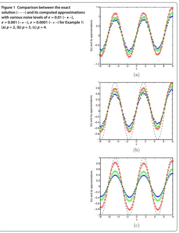
Figure 1 Comparison between the exact solution (– – –) and its computed approximations with various noise levels ofε= 0.01 (–∗–), ε= 0.001 (––),ε= 0.0001 (–◦–) for Example 1: (a)p= 2, (b)p= 3, (c)p= 4.
Moreover, we need to make the vectorgδ periodical [] and then we take the discrete
Fourier transform for the vectorgδ. The approximation of the regularization solution are
computed by using the fast Fourier transform algorithm [] and the range of the variable xin the numerical experiment is [–, ].
Example Consider a piecewise smooth source:
f(x) =
⎧ ⎪ ⎪ ⎪ ⎪ ⎪ ⎨ ⎪ ⎪ ⎪ ⎪ ⎪ ⎩
, –≤x≤–, x+ , – <x≤, –x+ , <x≤, , <x≤.
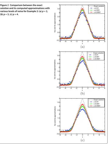
Figure 2 Comparison between the exact solution and its computed approximations with various levels of noise for Example 2: (a)p= 2, (b)p= 3, (c)p= 4.
Example Consider the following discontinuous case:
f(x) =
⎧ ⎪ ⎪ ⎪ ⎪ ⎪ ⎨ ⎪ ⎪ ⎪ ⎪ ⎪ ⎩
–, –≤x≤–, , – <x≤, –, <x≤, , <x≤.
(.)
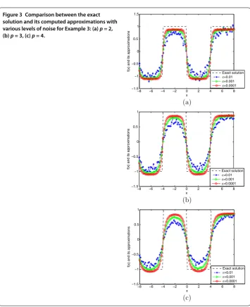
From Figures -, we can see that the smaller theε, the better the computed approx-imationfβ,δ(x). Aspincreases, the worse the computed approximation. This means the
Figure 3 Comparison between the exact solution and its computed approximations with various levels of noise for Example 3: (a)p= 2, (b)p= 3, (c)p= 4.
In Examples and , since the direct problem with the sourcef(x) does not have an analytical solution, the datag(x) is obtained by solving the direct problem. From Figures and , we can see that the numerical solutions are less ideal than that of Example . It is not difficult to see that the well-known Gibbs phenomenon and the recovered data near the non-smooth and discontinuities points are not accurate. Taking into consideration of the ill-posedness of the problem, the results presented in Figures and are reasonable.
6 Conclusions
Competing interests
The authors declare that they have no competing interests.
Authors’ contributions
All authors contributed equally to the writing of this paper. All authors read and approved the final manuscript.
Acknowledgements
The project is supported by the National Natural Science Foundation of China (No. 11171136, No. 11261032), the Distinguished Young Scholars Fund of Lanzhou University of Technology (Q201015) and the Basic Scientific Research Business Expenses of Gansu Province College.
Received: 15 October 2013 Accepted: 7 March 2014 Published:20 Mar 2014 References
1. Ahmadabadi, MN, Arab, M, Malek Ghaini, FM: The method of fundamental solutions for the inverse space-dependent heat source problem. Eng. Anal. Bound. Elem.33, 1231-1235 (2009)
2. Cannon, JR, Duchateau, P: Structural identification of an unknown source term in a heat equation. Inverse Probl.14, 535-551 (1998)
3. Yan, L, Fu, CL, Yang, FL: The method of fundamental solutions for the inverse heat source problem. Eng. Anal. Bound. Elem.32, 216-222 (2008)
4. Dou, FF, Fu, CL, Yang, FL: Optimal error bound and Fourier regularization for identifying an unknown source in the heat equation. J. Comput. Appl. Math.230, 728-737 (2009)
5. Wei, T, Zhang, ZQ: Reconstruction of a time-dependent source term in a time-fractional diffusion equation. Eng. Anal. Bound. Elem.37, 23-31 (2013)
6. Li, GS: Data compatibility and conditional stability for an inverse source problem in the heat equation. Appl. Math. Comput.173, 566-581 (2006)
7. Ma, YJ, Fu, CL, Zhang, YX: Identification of an unknown source depending on both time and space variables by a variational method. Appl. Math. Model.36, 5080-5090 (2012)
8. Yang, L, Deng, ZC, Yu, JN, Luo, GW: Optimization method for the inverse problem of reconstructing the source term in a parabolic equation. Math. Comput. Simul.80, 314-326 (2009)
9. Yang, F, Fu, CL: Two regularization methods to identify time-dependent heat source through an internal measurement of temperature. Math. Comput. Model.53, 793-804 (2011)
10. Ohe, T, Ohnaka, K: A precise estimation method for locations in an inverse logarithmic potential problem for point mass models. Appl. Math. Model.18, 446-452 (1994)
11. Nara, T, Ando, S: A projective method for an inverse source problem of the Poisson equation. Inverse Probl.19, 355-369 (2003)
12. Farcas, A, Elliott, L, Ingham, DB, Lesnic, D, Mera, NS: A dual reciprocity boundary element method for the regularized numerical solution of the inverse source problem associated to the Poisson equation. Inverse Probl. Sci. Eng.11(2), 123-139 (2003)
13. Kagawa, Y, Sun, Y, Matsumoto, O: Inverse solution of Poisson equation using DRM boundary element models -identification of space charge distribution. Inverse Probl. Sci. Eng.1(2), 247-265 (1995)
14. Sun, Y, Kagawa, Y: Identification of electric charge distribution using dual reciprocity boundary element models. IEEE Trans. Magn.33(2), 1970-1973 (1997)
15. Jin, BT, Marin, L: The method of fundamental solutions for inverse source problems associated with the steady-state heat conduction. Int. J. Numer. Methods Eng.69, 1570-1589 (2007)
16. Lattés, R, Lions, JL: The Method of Quasireversibility: Applications to Partial Differential Equations. Elsevier, New York (1969)
17. Showalter, RE, Ting, TW: Pseudo-parabolic partial differential equations. SIAM J. Math. Anal.1(1), 1-26 (1970) 18. Miller, K: Stabilized quasireversibility and other nearly best possible methods for non-well posed problems. In:
Symposium on Non-Well-Posed Problems and Logarithmic Convexity. Lecture Notes in Math., vol. 316, pp. 161-176. Springer, Berlin (1973)
19. Mel’nikova, IV: Regularization of ill-posed differential problems. Sib. Math. J.33(2), 289-298 (1992)
20. Ames, KA, Cobb, SS: Continuous dependence on modeling for related Cauchy problems of a class of evolution equations. J. Math. Anal. Appl.215(1), 15-31 (1997)
21. Huang, Y, Zheng, Q: Regularization for a class of ill-posed Cauchy problems. Proc. Am. Math. Soc.133(10), 3005-3012 (2005)
22. Denche, M, Bessila, K: A modified quasi-boundary value method for ill-posed problems. J. Math. Anal. Appl.301(2), 419-426 (2005)
23. Boussetila, N, Rebbani, F: Optimal regularization method for ill-posed Cauchy problems. Electron. J. Differ. Equ.2006, 147 (2006)
24. Showalter, RE: Cauchy problem for hyperparabolic partial differential equations. In: Trends in the Theory and Practice of Non-Linear Analysis, pp. 421-425. Elsevier, Amsterdam (1983)
25. Feng, XL, Eldén, L, Fu, CL: A quasi-boundary-value method for the Cauchy problem for elliptic equations with nonhomogeneous Neumann data. J. Inverse Ill-Posed Probl.18(6), 617-645 (2010)
26. Eldén, L, Berntsson, F, Regi `nska, T: Wavelet and Fourier methods for solving the sideways heat equation. SIAM J. Sci. Comput.21, 2187-2205 (2000)
27. Kirsch, A: An Introduction to the Mathematical Theory of Inverse Problems. Springer, New York (1996) 28. Engl, HW, Hanke, M, Neubauer, A: Regularization of Inverse Problem. Kluwer Academic, Boston (1996)
10.1186/1029-242X-2014-117