Multi objective multi item solid transportation problem with fuzzy inequality constraints

R E S E A R C H

Open Access

Multi-objective multi-item solid

transportation problem with fuzzy inequality

constraints

Dipankar Chakraborty

_{, Dipak Kumar Jana}

_{and Tapan Kumar Roy}

*_{Correspondence:}

[email protected]

2_{Department of Applied Science,}

Haldia Institute of Technology, Purba Midnapur, Haldia, West Bengal 721657, India Full list of author information is available at the end of the article

Abstract

Zimmermann (Int. J. Gen. Syst. 2:209-215, 1976) first introduced the concept of fuzzy inequality in the field of linear programming problem (LPP). But this concept is hardly used in any real life applications of LPP. So, in this paper, a multi-objective multi-item solid transportation problem (MMSTP) with fuzzy inequality constraints is modeled. Representing different preferences of the decision maker for transportation, three different types of models are formulated and analyzed. Fuzzy inequality solid

transportation problem is converted to parameter solid transportation problem by an appropriate choice of flexible index, and then the crisp solid transportation problem is solved by the algorithm (Cao in Optimal Models and Methods with Fuzzy Quantities, 2010) for decision values. Fuzzy interactive satisfied method (FISM), global criterion method (GCM) and convex combination method (CCM) are applied to derive optimal compromise solutions for MMSTP by using MatLab and Lingo-11.0. The models are illustrated with numerical examples and some sensitivity analysis is also presented.

Keywords: solid transportation problem; fuzzy inequality; global criterion method; fuzzy interactive satisfied method; convex combination method

1 Introduction

The solid transportation problem (STP) is a generalization of the traditional transporta-tion problem in which three-dimensional properties (supply, demand, convenience) are taken into account in the objective and constraint set instead of source and destination. The necessity of considering this special type of transportation problem arises when het-erogeneous conveyances are available for shipment of products. The STP is used in public distribution systems. In many industrial problems, a homogeneous product is delivered from its origin to a destination by means of different modes of transport called con-veyances, such as trucks, cargo flights, goods trains, ships,etc. These conveyances are taken as the third dimension. A solid transportation problem can be converted to a clas-sical transportation problem by considering only a single type of conveyance.

The STP was first introduced by Haley [] in . In recent years, there have been numerous papers in this area. Some papers only minimize the total transportation cost. For example, Ojhaet al.[], Pramaniket al.[] considered an STP for an item with fixed charge, vehicle cost and price discounted varying charge. However, in practical program-ming problems, the decision maker (DM) usually needs to optimize several objectives.

Thus, the DM cannot obtain the optimal values of all the objectives simultaneously. The growing literature of STP focuses on multiple objective problems, that is, multiple objec-tive solid transportation problems (MOSTPs). For example, Bitet al.[] used a fuzzy pro-gramming approach to solve a MOSTP; Idaet al.[] presented a neural network method to solve a MOSTP; Gao and Liu [] developed two-phase fuzzy algorithms to solve multi-objective STP; Tao and Xu [] developed a class of rough multiple multi-objective programming and its application to a solid transportation problem.

If more than one objective is to be optimized in an STP, then the problem is called multi-objective solid transportation problem (MOSTP). If we consider more than one item, then it is called multi-item solid transportation problem. If we consider more than one item and more than one objective at a time in an STP, then it is called a objective multi-item solid transportation problem (MMSTP). The MMSTP model was given by Kundu

et al.[]. Recently, Pramaniket al.[] have developed a multi-objective STP in a fuzzy random environment.

Nowadays, in a very often changing market, the business of a single item does not pay much profit to a retailer. For this reason, almost all businessmen in the fields of transporta-tion (Sancak and Salman []) do the business of several items. Generally, in all the cases of STP (multi-objective, multi-item and multi-objective multi-item ones), the inequality has been considered as a general inequality. But we can consider this inequality in the fuzzy environment named fuzzy inequality [, ]. Fuzzy inequality means it will essen-tially satisfy that inequality condition. Flexible index is used (Cao []) to convert it into the general inequality, so that it will give you a chance to choose the appropriate decision value. Two algorithms were given by Cao [] to find the decision value. We have taken one of them to find the decision value. That decision value will give us a more general optimal solution and an optimal value to minimize the objectives.

The following developments are made in the formulation and solution of MMSTP mod-els:

• Various types of examples have been used to illustrate the single-objective fuzzy inequality constraints.

• MMSTP has been solved in a fuzzy inequality constraint environment.

• Three different soft computing techniques FISM, GCM and CCM have been used to make the comparison between optimal solutions in multi-objective problems. • Two different soft-computing tools (MATLAB and LINGO-.) have been used to

solve the examples.

2 Preliminaries about fuzzy inequality constraint linear programming Let us consider the fuzzy inequality constraint linear programming (FICP)

maxz=cx

LP s.t.Axb, ()

x≥,

its corresponding parameter linear programming is given by (Cao [])

maxz=cx

LPα s.t.Ax≤b+ ( –α)d, ()

x≥,

whereα∈[, ] andd≥. In the given discussion, we will usexαas an optimal solution, Bαdenotes an optimal basis andzαdenotes an optimal value of linear programming (LPα).

Definition .[] Let Bbe one of the optimal basis matrices of (LPα). If an interval

[α,α] exists, satisfying thatBis an optimal basis matrix of (LPα) (∀α∈[α,α]) while Bis not an optimal basis matrix for eachα∈/ [α,α], we callαandαcritical values of

(LPα) and [α,α] a characteristic interval.

Theorem  (LPα)has a finite characteristic interval on the interval[, ].

Theorem  Let B be an optimal basis matrix of(LPα)on a characteristic interval[α,α]. If(B–_b)

i=  (≤i≤m),then

α=max

[B–_(b+d)]

i [B–_b]

i

, B–d_i<  (≤i≤m)

,

α=min

[B–_(b+d)]

i [B–_b]

i

, B–d_i>  (≤i≤m)

are derived,where(B–(b+d))iand(B–d)iare the ith components of B–(b+d)and B–d,

respectively.

Property . LetBbe an optimal matrix of (LPα) on the characteristic interval [αi,αj]. Thenxα=B–(b+ ( –α)d) (αi≤α≤αj) is a linear vector function about variableα. The optimal value functionzα=CBB–(b+ ( –α)d) is a linear function about variableαand decreases with the increase of variableα.

Property . The optimal value of functionzαof (LPα) continues on the interval [, ]. 2.1 Algorithm for fuzzy inequality constraint linear programming

Step : Let the optimal solutions of (LP) and (LP) bexand x, the optimal values of (LP) and (LP) bezandz, and the optimal basis matrix of (LP) beB.

Step : Solve[B–

(b+ ( –α)d)]i= . Assume the solution as

α,α, . . . ,αn– ( <α<α<· · ·<αn–< ).

Letα= ,αn= ,α=α,k= .

Step : Solve (LPα).

Let the optimal value beZα. IfZα≤Z+dα, turn to Step , otherwise letk=k+ ,

α=αk, turn to Step . Step : Solve the optimal decision

α∗=Zαk–Zαk––Zαk–αk+Zαkαk– Zαk–Zαk––αkd+αk–d

.

Step : Solve linear programming (LPα∗), and we can obtain an optimal solutionxα∗ and

an optimal valuezα∗.

Example . Calculate maxx+ x+ x

subject to

x+ x+ x,

x+x+x,

LP x+x,

x,

x+x,

x,x,x≥,

()

whered= (, , , , ).

The corresponding parametric linear programming problem of the aboveLP is pre-sented as follows:

maxx+ x+ x

subject to

x+ x+ x≤,

x+x+x≤,

LPα x+x≤,

x≤,

x+x≤ + ( –α),

≤α≤, x,x,x≥.

Now, using algorithm given in Section ., we obtainZ= .,Z=  andd= . by calculating (LP) and (LP). The inverse of the optimal matrix in (LP) is

B–_ = ⎛ ⎜ ⎜ ⎜ ⎜ ⎜ ⎜ ⎝

. –.   . .    –.

–. .   –. –.    . –. .   –.

⎞ ⎟ ⎟ ⎟ ⎟ ⎟ ⎟ ⎠ .

Now, calculating the equations [B–

(, , , , –α)]i=  (i= , , . . . , ), respectively, we obtainα= .,α= ., assumeα=  andα= .

Now solving (LPα) we get the optimal solution asx= .,x= . andx= 

and the optimal value asZα=Z.= ..

SinceZ.= . >Z+ .∗. = ., we must continue to solve the linear programming (LPα). By solving (LPα), we obtain the optimal solution asx= ., x=  andx=  and the optimal value asZα=Z.= .

NowZ.=  <Z+ .∗. = ., so we stop here and calculate optimal decisionα∗.

Now

α∗=Zα–Zα–Zαα+Zαα Zα–Zα–αd+αd

= ..

Now calculating (LP.), we obtain the optimal solution asx= .,x= .

andx=  and the optimal value asZ∗_{.}= ..

3 Notations and assumptions

3.1 Notations

In this solid transportation problem, the following notations are used: (i) M=number of sources of the transportation problem. (ii) N=number of destinations of the transportation problem. (iii) K=number of conveyances,i.e., different modes of transportation. (iv) ap_i =amount of product available atith origin forpth item.

(v) bp_j =demand atjth destination ofpth item. (vi) ek=conveyances of the transportation problem. (vii) T =number of items.

(viii) xp_ijk =the amount to be transported fromith origin tojth destination by means of

kth conveyance ofpth item (decision variables).

(ix) C_ijktp=per unit transportation cost fromith origin tojth destination bykth conveyance ofpth item andtth objective.

3.2 Assumptions

In this solid transportation problem, the following assumptions are made. (i) Homogeneous product should be transported from sources to destinations. (ii) During transportation no items are damaged,i.e., the amount of received items in

4 Multi-objective multi-item LPP with fuzzy inequality constraint

Consider the following multi-objective linear programming problems with fuzzy con-straint:

⎧ ⎪ ⎨ ⎪ ⎩

minxC_l(p)x(p), l= , , . . . ,kandp= , , . . . ,T

s.t.

A(_ip)(x(p)_)B(p)

i , i= , , . . . ,rand∀p,

x(p)_{≥ ∀p,}

()

wherexis ann-dimensional decision variable column vector. Its corresponding parametric linear programming is given by

⎧ ⎪ ⎨ ⎪ ⎩

minxCl(p)x(p), l= , , . . . ,kandp= , , . . . ,T

s.t.

A(_ip)(x(p)_)≤B(p)

i +Vi, i= , , . . . ,rand∀p,

x(p)_{≥ ∀p,}

()

whereVi(≤i≤r) is a flexible index by an appropriate choice.

Now the solution methodology of a multi-objective decision making problem by con-verting into a single-objective problem is discussed as follows.

4.1 Fuzzy interactive satisfied method

We introduce the interactive fuzzy satisfied method (FISM) proposed by Sakawa [], Xu and Zhou []. We consider the following multi-objective decision-making model:

max[Gi(x),i= , , . . . ,M]

s.t.x∈X. ()

The objective function of equation () is to maximizeGi(x), so for each objective we intro-duce the fuzzy objective ‘Gi(x) approximately more than some value’, and the membership function is

μi

Gi(x)

= ⎧ ⎪ ⎪ ⎨ ⎪ ⎪ ⎩

 forGi(x) >Gi,

 –Gi(x)–Gi

G i–Gi

forG

i ≤Gi(x)≤Gi,  forGi(x) <Gi.

()

In equation (), the membership is  and  when the values ofGi(x) areGiandGi, respec-tively,

G_i=max

x∈X Gi(x), G



i =min_x∈XGi(x), i= , , . . . ,M. ()

For modelminx∈XGi(x), its optimal solution should be gotten at the boundary of the con-vex setX. If there exists no solution ofmaxx∈XGi(x) orminx∈XGi(x), orGi=∞,Gi = –∞, the decision maker may set the value ofG

i,Gi subjectively. Hence, equation () could be transformed into the following form:

min[μ(G(x)),μ(G(x)), . . . ,μm(GM(x))]

For each objective functionμ(Gi(x)), let the decision maker give the reference value of membership functionμ¯ito reflect the ideal value of membership function. Through solv-ing the minmax problem (), we obtain an efficient solution of equation () as follows:

min max_{i=,,...,M}[μ¯i–μi(Gi(x))]

s.t.x∈X. ()

Equation () is equivalent to ⎧

⎪ ⎨ ⎪ ⎩

minλ

s.t.

¯

μi–μi(Gi(x))≤λ, j= , , . . . ,p, ≤λ≤, x∈X.

()

4.2 Global criteria method

The global criteria method gives a compromise solution for a multi-objective problem. Ac-tually this method is a way of achieving compromise in minimizing the sum in derivations of the ideal solutions from the respective objective functions. The solution procedure is as follows.

Step-I: Solve the multi-objective problem using each time only one objective ft (t= , , . . . ,R) ignoring all the other objectives.

Step-II: From the results of Step-I, determine the ideal objective vector, say(fmin  ,fmin,

. . . ,fmin

R )and the corresponding values of(fmax,fmax, . . . ,fRmax). Step-III: Formulate the following auxiliary problem:

minG(x)

subject togj(x)≤, j= , , . . . ,M,

x≥,

where G(x) =min{R_t=(ft(x)–ftmin

ftmin

)q_}q _{or G(x) =min}{R

t=(

ft(x)–ftmin

ftmax–ftmin

)q_}q_{, where}

≤q<∞. A usual value ofq is . This method is then called global criteria method inLnorms.

4.3 Convex combination method

We consider the following multi-objective model: ⎧

⎪ ⎨ ⎪ ⎩

min[fi(x),i= , , . . . ,M] s.t.gj≥, j= , , . . . ,N,

x∈X.

()

Then, by the convex combination method, we transfer the above problem into the follow-ing form:

⎧ ⎪ ⎨ ⎪ ⎩

minM_i=wifi(x), where M

i=wi= ,  <wi<  s.t.gj≥, j= , , . . . ,N,

x∈X.

()

5 Formulation of different models of STP

5.1 Model-1: multi-objective multi-item STP

Letp(p= , , . . . ,T) items be transported fromMorigins (or sources)ai(i= , , . . . ,M),N destinations (i.e., demands)bj(j= , , . . . ,N) andKconveyancesek(k= , , . . . ,K).K con-veyances, i.e., different modes of transport, may be trucks, cargo flights, goods trains, ships,etc.Leta(_ip)be the product available atith origin for itemsp(p= , , . . . ,T),b(_jp)be the demand atjth destination for itemsp(p= , , . . . ,T), and letekrepresent the amount of product which can be carried bykth conveyance. The variablex(_ijkp)represents the un-known quantity to be transported from origina(_ip)to destinationb(_jp)by means ofkth con-veyance for itemp= , , . . . ,T. Then we propose the mathematical model for the fuzzy inequality constraint. Single-objective and p(= , , . . . ,T)-item problem is to minimize the total transportation cost as follows:

ft(p)= M

i=

N

j=

K

k=

c_ijk(tp)x_ijk(p) ∀pand∀t. ()

From the discussion above, we develop mathematical formulations of the objectives as follows:

minft= T

p=

M

i=

N

j=

K

k=

c(_ijktp)x(_ijkp) ∀t. ()

As mentioned by Haley [], the constraints are divided into three types: source constraint, destination constraint and conveyance capacity constraint. In the fuzzy environment, the quantity from a source is essentially less than equal to the supply capacity of products for different items, that is,

N

j=

K

k=

x_ijk(p)a_i(p), i= , , , . . . ,M∀p. ()

In the fuzzy environment, the quantity of product transported to a destination is essen-tially greater than equal to its demand for different items, that is,

M

i=

K

k=

x_ijk(p)b_j(p), j= , , , . . . ,N∀p. ()

In the fuzzy environment, the transportation quantity of conveyance is essentially less than equal to its capacity, that is,

T

p=

M

i=

N

j=

x(_ijkp)ek, k= , , , . . . ,K. ()

It is natural to require the nonnegativity of decision variablex(_ijkp), that is,

x(_ijkp)≥ ∀i,j,kand∀p. ()

while the modeling analyst may be an expert in transportation problems or a researcher in the enterprise. With the complexity of feasible region, the DM may give an appropriately large region so that all the feasible solutions are included in it. Hence, the above MMSTP with fuzzy inequality constraint can be written as

minft=min T

p=

M

i=

N

j=

K

k=

c(_ijktp)x(_ijkp), t= , , . . . ,R

s.t. N

j=

K

k=

x_ijk(p)a_i(p), i= , , , . . . ,M∀p,

M

i=

K

k=

x_ijk(p)b_j(p), j= , , , . . . ,N∀p, ()

T

p=

M

i=

N

j=

x(_ijkp)ek, k= , , , . . . ,K,

x(_ijkp)≥ ∀i,j,k,

wheremeans ‘essentially smaller than equal to’ andmeans ‘essentially greater than equal to’.

5.2 Model-2: multi-objective single-item STP

We consider a multi-objective single-item solid transportation problem with fuzzy in-equality constraint. Then the model may be written as

minft=min M

i=

N

j=

K

k= ctp_ijkxijk

s.t. N

j=

K

k=

xijkai, i= , , , . . . ,M,

M

i=

K

k=

xijkbj, j= , , , . . . ,N, ()

M

i=

N

j=

xijkek, k= , , , . . . ,K,

xijk≥ ∀i,j,k.

5.3 Model-3: single-objective multi-item STP

We consider a single-objective multi-item solid transportation problem with fuzzy in-equality constraint. Then the model may be written as

minf =min T

p=

M

i=

N

j=

K

k= c(_ijkp)x(_ijkp)

s.t. N

j=

K

k=

M i= K k=

x_ijk(p)b_j(p), j= , , , . . . ,N∀p, ()

T p= M i= N j=

x(_ijkp)ek, k= , , , . . . ,K,

x(_ijkp)≥ ∀i,j,k.

6 Solution of proposed models

6.1 Model-1

Let us consider thatpdifferent items are to be transported fromith origin tojth destina-tion by means ofkth conveyance. Here we have considered a two-objective function. Let max_x∈Xf=fU,minx∈Xf=fL,maxx∈Xf=fU andminx∈Xf=fL. Then the membership

functions offandfare given by

μ

f(x)

= ⎧ ⎪ ⎪ ⎨ ⎪ ⎪ ⎩

 forf(x) >f_U, f_U–f(x)

fU–fL

forfL

 <f(x) <fU,

 forf(x) <fL

,

μ

f(x)

= ⎧ ⎪ ⎪ ⎨ ⎪ ⎪ ⎩

 forf(x) >f_U, f_U–f(x)

fU–fL

forfL

 <f(x) <fU,

 forf(x) <fL

.

Now, using FISM in Section ., we present the equivalent crisp linear programming of () as follows:

⎧ ⎪ ⎪ ⎪ ⎪ ⎪ ⎪ ⎪ ⎪ ⎪ ⎪ ⎪ ⎪ ⎪ ⎪ ⎨ ⎪ ⎪ ⎪ ⎪ ⎪ ⎪ ⎪ ⎪ ⎪ ⎪ ⎪ ⎪ ⎪ ⎪ ⎩

min_xλ

s.t. ⎧ ⎪ ⎪ ⎪ ⎪ ⎪ ⎪ ⎪ ⎪ ⎪ ⎪ ⎪ ⎪ ⎨ ⎪ ⎪ ⎪ ⎪ ⎪ ⎪ ⎪ ⎪ ⎪ ⎪ ⎪ ⎪ ⎩

f≤f_U– (μ–λ)(fU–fL), f≤fU

 – (μ–λ)(fU–fL),

N j=

K k=x

(p)

ijk ≤a

(p)

i + ( –α)d

(p)

i , i= , , , . . . ,M, M

i=

K k=x

(p)

ijk ≥b

(p)

j + ( –α)v

(p)

j , j= , , , . . . ,N, T

p=

M i=

N j=x

(p)

ijk ≤ek+ ( –α)uk, k= , , , . . . ,K, ≤α≤,

x(_ijkp)≥ ∀i,j,kand∀p.

6.2 Model-2

Letmaxx∈Xf=fU,minx∈Xf=fL,maxx∈Xf=fUandminx∈Xf=fL. Then the membership

functions offandfare given by

μ

f(x)= ⎧ ⎪ ⎪ ⎨ ⎪ ⎪ ⎩

 forf(x) >fU,

fU –f(x)

f_U–f_L forf L

 <f(x) <fU,

 forf(x) <fL,

μ

f(x)= ⎧ ⎪ ⎪ ⎨ ⎪ ⎪ ⎩

 forf(x) >fU

 ,

f_U–f(x)

f_U–f_L forf L

 <f(x) <fU,

Now, using FISM in Section ., we present the equivalent crisp linear programming of () as follows:

⎧ ⎪ ⎪ ⎪ ⎪ ⎪ ⎪ ⎪ ⎪ ⎪ ⎪ ⎪ ⎪ ⎪ ⎪ ⎨ ⎪ ⎪ ⎪ ⎪ ⎪ ⎪ ⎪ ⎪ ⎪ ⎪ ⎪ ⎪ ⎪ ⎪ ⎩

minxλ

s.t. ⎧ ⎪ ⎪ ⎪ ⎪ ⎪ ⎪ ⎪ ⎪ ⎪ ⎪ ⎪ ⎪ ⎨ ⎪ ⎪ ⎪ ⎪ ⎪ ⎪ ⎪ ⎪ ⎪ ⎪ ⎪ ⎪ ⎩

f≤f_U– (μ–λ)(fU–fL), f≤fU

 – (μ–λ)(fU–fL),

N j=

K

k=xijk≤ai+ ( –α)di, i= , , , . . . ,M, M

i=

K

k=xijk≥bj+ ( –α)vj, j= , , , . . . ,N M

i=

N j=x

(p)

ijk ≤ek+ ( –α)uk, k= , , , . . . ,K, ≤α≤,

x(_ijkp)≥ ∀i,j,k.

6.3 Model-3

Now corresponding parametric linear programming of equation () is presented as fol-lows: min T p= M i= N j= K k= c(_ijkp)x(_ijkp)

s.t. N j= K k=

x(_ijkp)≤a(_ip)+ ( –α)d(_ip), i= , , , . . . ,Mand∀p,

M i= K k=

x(_ijkp)≥b(_jp)+ ( –α)v(_jp), j= , , , . . . ,Nand∀p, ()

T p= M i= N j=

x(_ijkp)≤ek+ ( –α)uk, k= , , , . . . ,K,

≤α≤, xijk≥ ∀i,j,k,

whered(_ip)fori= , , , . . . ,M,v_jpforj= , , , . . . ,Nandukfork= , , , . . . ,Kare flexible index values∀p.

7 Numerical experiment

7.1 Input data for Model-1 and Model-3

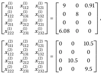
Let us consider a multi-objective multi-item solid transportation problem with two types of items (i.e.,T= ), three origins (i.e.,M= ), two destinations (i.e.,N= ) and two types of conveyances (i.e.,K= ). The parameters are given as follows.

Transportation cost forst objective andst item[c()_ijk ]

⎡ ⎢ ⎢ ⎢ ⎣

c()_ c()_ c()_ c()_ c()_ c()_ c()_ c()_ c()_ c()_ c()_ c()_

Transportation cost forst objective andnd item[c()_ijk ] ⎡ ⎢ ⎢ ⎢ ⎣

c()_ c()_ c()_ c()_ c()_ c()_ c()_ c()_ c()_ c()_ c()_ c()_

⎤ ⎥ ⎥ ⎥ ⎦= ⎡ ⎢ ⎢ ⎢ ⎣             ⎤ ⎥ ⎥ ⎥ ⎦.

Transportation cost fornd objective andst item[c()_ijk ] ⎡

⎢ ⎢ ⎢ ⎣

c()_ c()_ c()_ c()_ c()_ c()_ c() c

()

 c

()  c()_ c()_ c()_

⎤ ⎥ ⎥ ⎥ ⎦= ⎡ ⎢ ⎢ ⎢ ⎣             ⎤ ⎥ ⎥ ⎥ ⎦.

Transportation cost fornd objective andnd item[c()_ijk ] ⎡

⎢ ⎢ ⎢ ⎣

c() c ()

 c

()  c()_ c()_ c()_ c()_ c()_ c()_ c()_ c()_ c()_

⎤ ⎥ ⎥ ⎥ ⎦= ⎡ ⎢ ⎢ ⎢ ⎣             ⎤ ⎥ ⎥ ⎥ ⎦.

Amount of items available at origin[ap_i]

a()_ a()_ a()_ a()_

=     .

The demand amount of items at destination[b(_jp)]

b()_ b()_ b()_ b()_ b()_ b()_

=       .

Amount of items transported by conveyances[ck]

[e e] = [ ].

Optimum result for Model-

With the above input data,fandfare calculated using GRG, and we get

f_U= ., f_L= ., f_U= ,, f_L= .

So, we can get the membership functions offandf(Figure ) as follows:

μ

f(x)

= ⎧ ⎪ ⎨ ⎪ ⎩

 forf(x) > .,

.–f(x)

.–. for . <f(x) < .,

 forf(x) < .,

μ

f(x)= ⎧ ⎪ ⎨ ⎪ ⎩

 forf(x) > ,,

,–f(x)

,– for , <f(x) < ,

Figure 1 Membership functions off1andf2.

Table 1 Employ the interactive fuzzy satisfied method based on the fuzzy inequality constraint of Model-1

μ1 μ2 f1 f2 μ1(f1) μ2(f2) Values of decision variables λ

1 1 634.3 826.09 0.641 0.641 x1

111= 9,x1211 = 2.04,x1131= 8,x1222= 4.95,

x2

121= 9.45,x1222 = 1.04,x2122 = 10.5,x2322 = 9.50

0.35

1 0.9 630.98 853.13 0.679 0.579 x1

111= 9,x1211 = 3.17,x1131= 8,x1222= 3.82,

x2121= 8.32,x1222 = 2.17,x2122 = 10.5,x2322 = 9.5

0.32

0.9 1 637.76 799.15 0.603 0.703 x1111= 9,x1211 = 0.91,x1131= 8,x1222= 6.08,

x2

121= 10.5,x2122 = 10.5,x2322 = 9.5

0.296

Then we compute the following model to get the interactive satisfied solution:

⎧ ⎪ ⎪ ⎪ ⎪ ⎪ ⎪ ⎪ ⎪ ⎪ ⎪ ⎪ ⎪ ⎪ ⎪ ⎪ ⎪ ⎪ ⎪ ⎪ ⎪ ⎪ ⎪ ⎪ ⎪ ⎪ ⎪ ⎪ ⎪ ⎪ ⎪ ⎪ ⎪ ⎪ ⎪ ⎪ ⎪ ⎪ ⎨ ⎪ ⎪ ⎪ ⎪ ⎪ ⎪ ⎪ ⎪ ⎪ ⎪ ⎪ ⎪ ⎪ ⎪ ⎪ ⎪ ⎪ ⎪ ⎪ ⎪ ⎪ ⎪ ⎪ ⎪ ⎪ ⎪ ⎪ ⎪ ⎪ ⎪ ⎪ ⎪ ⎪ ⎪ ⎪ ⎪ ⎪ ⎩

minxλ

s.t. ⎧ ⎪ ⎪ ⎪ ⎪ ⎪ ⎪ ⎪ ⎪ ⎪ ⎪ ⎪ ⎪ ⎪ ⎪ ⎪ ⎪ ⎪ ⎪ ⎪ ⎪ ⎪ ⎪ ⎪ ⎪ ⎪ ⎪ ⎪ ⎪ ⎪ ⎪ ⎪ ⎪ ⎪ ⎪ ⎪ ⎨ ⎪ ⎪ ⎪ ⎪ ⎪ ⎪ ⎪ ⎪ ⎪ ⎪ ⎪ ⎪ ⎪ ⎪ ⎪ ⎪ ⎪ ⎪ ⎪ ⎪ ⎪ ⎪ ⎪ ⎪ ⎪ ⎪ ⎪ ⎪ ⎪ ⎪ ⎪ ⎪ ⎪ ⎪ ⎪ ⎩

(. –f(x))≥(μ–λ)(. – .),

(, –f(x))≥(μ–λ)(, – ), x

+x+x+x+x+x≤, x

+x+x+x+x+x≤, x

+x+x+x≥, x+x+x+x≥, x_+x_+x_+x_≥,

x

+x+x+x+x+x≤, x

+x+x+x +x+x≤ + ( –a), x

+x+x +x≥ + ( –α), x_+x_+x_+x_≥ + ( –α),

x

+x+x +x≥ + ( –α), x

+x+x+x +x+x+x

+x

+x+x+x+x≤ + ( –α), x+x+x+x+x+x+x

+x_+x_+x_+x_+x_≤ + ( –α), ≤α≤, xijk≥ ∀i,j,k,

whereα= . has been calculated in Example .. Here we solve Model-, to get the sat-isfied solutions, which are listed in Table .

The first line of Table  lists each reference value of membership functionμ(f), when

Table 2 Optimum results by using the convex combination method of Model-1

w1 w2 f1 f2 Values of decision variables

0.5 0.5 691.5 670 x1

111= 9,x1131= 6.5,x2221 = 7,x1232= 1.5,x2212= 10.5,x2222= 10.5,x2231= 9.5

0.6 0.4 688 673.5 x1

111= 9,x1131= 8,x2221 = 7,x2212= 10.5,x2221= 2,x2222 = 8.5,x2312 = 9.5

0.7 0.3 651 748.5 x1111= 9,x1131= 8,x2221 = 7,x2212= 10.5,x2221= 10.5,x2232= 9.5

Table 3 Comparison of optimum results of Model-1

Method f1 f2 Values of decision variables

FISM 630.98 799.15 x1

111= 9,x1121= 0.91,x1311 = 8,x1222= 6.08,

x2121= 10.5,x2212= 10.5,x2232= 9.5

Convex combination 651 748.5 x1111= 9,x1311 = 8,x2221 = 7,x2212= 10.5,

x2221= 10.5,x2232= 9.5

Global criteria 669 711.2 x1

111= 9,x1131= 6.75,x2221 = 7,x1232= 1.24,

x2

221= 7.95,x2212= 10,x2231= 4.78,

x1

222= 2.54,x2232= 4.71,GC= 0.1265

f(x), we may consider resetting the reference value of membership function (μ,μ),e.g.,

we set (μ,μ) = (., ) or (μ,μ) = (, .). The corresponding results are listed in the

second and third lines. Suppose that when the reference value of membership function is (μ,μ) = (., ), the decision maker is satisfied, then the interactive process is stopped,

so we obtain that the satisfied solutions for different items are

⎡ ⎢ ⎢ ⎢ ⎣

x()_ x()_ x()_ x()_ x()_ x()_ x()_ x()_ x()_ x()_ x()_ x()_

⎤ ⎥ ⎥ ⎥ ⎦=

⎡ ⎢ ⎢ ⎢ ⎣

  .

  

  

.   ⎤ ⎥ ⎥ ⎥ ⎦,

⎡ ⎢ ⎢ ⎢ ⎣

x()_ x()_ x()_ x()_ x()_ x()_ x()_ x()_ x()_ x()_ x()_ x()_

⎤ ⎥ ⎥ ⎥ ⎦=

⎡ ⎢ ⎢ ⎢ ⎣

  .

  

 . 

  .

⎤ ⎥ ⎥ ⎥ ⎦

and the corresponding optimal values for different items are

f_() f_() f_() f_()

=

. . . 

.

Applying the convex combination method stated in Section ., we get Table  for different weights onfandf. The comparison between the optimum results calculated by different methods for Model- is given in Table .

7.2 Input data for Model-2

Transportation cost forst objective[c()_ijk] ⎡

⎢ ⎢ ⎢ ⎣

c()_ c()_ c()_ c()_ c()_ c()_ c()_ c()_ c()_ c()_ c()_ c()_

⎤ ⎥ ⎥ ⎥ ⎦=

⎡ ⎢ ⎢ ⎢ ⎣

            ⎤ ⎥ ⎥ ⎥ ⎦.

Transportation cost fornd objective[c()_ijk] ⎡

⎢ ⎢ ⎢ ⎣

c()_ c()_ c()_ c()_ c()_ c()_ c()_ c()_ c()_ c()_ c()_ c()_

⎤ ⎥ ⎥ ⎥ ⎦=

⎡ ⎢ ⎢ ⎢ ⎣

            ⎤ ⎥ ⎥ ⎥ ⎦.

Amount of items available at origin[ai]

[a a] = [ ].

The demand amount of items at destination[bj]

[b b b] = [  ].

Amount of items transported by conveyances[ck]

[e e] = [ ].

Optimum result for Model-

With the above input data,fandfare calculated using the GRG technique, and we get

f_U= ., f_L= ., f_U= ., f_L= ..

So we can get the membership functions offandf(Figure ) as follows:

μ

f(x)= ⎧ ⎪ ⎨ ⎪ ⎩

 forf(x) > ., .–f(x)

.–. for . <f(x) < .,

 forf(x) < .,

μ

f(x)

=

⎧ ⎪ ⎨ ⎪ ⎩

 forf(x) > .,

.–f(x)

.–. for . <f(x) < .,

 forf(x) < ..

Then we compute the following model to get the interactive satisfied solution: ⎧

⎪ ⎪ ⎪ ⎪ ⎪ ⎪ ⎪ ⎪ ⎪ ⎪ ⎪ ⎪ ⎪ ⎪ ⎪ ⎪ ⎪ ⎪ ⎪ ⎪ ⎨ ⎪ ⎪ ⎪ ⎪ ⎪ ⎪ ⎪ ⎪ ⎪ ⎪ ⎪ ⎪ ⎪ ⎪ ⎪ ⎪ ⎪ ⎪ ⎪ ⎪ ⎩

min_xλ

s.t. ⎧ ⎪ ⎪ ⎪ ⎪ ⎪ ⎪ ⎪ ⎪ ⎪ ⎪ ⎪ ⎪ ⎪ ⎪ ⎪ ⎪ ⎪ ⎪ ⎨ ⎪ ⎪ ⎪ ⎪ ⎪ ⎪ ⎪ ⎪ ⎪ ⎪ ⎪ ⎪ ⎪ ⎪ ⎪ ⎪ ⎪ ⎪ ⎩

(. –f(x))≥(μ–λ)(. – .),

(. –f(x))≥(μ–λ)(. – .), x+x+x+x+x+x≤,

x+x+x+x+x+x≤,

x+x+x+x≥ + ( –α),

x+x+x+x≥ + ( –α),

x+x+x+x≥ + ( –α),

x+x+x+x+x+x≤ + ( –α),

x+x+x+x+x+x≤ + ( –α),

xijk≥ ∀i,j,k, ≤α≤,

whereα= . has been already calculated in Example .. Here we solve Model- to get the satisfied solutions, which are listed in Table .

The first line of Table  lists each reference value of membership functionμ(f), when

the initialized membership function is , the value of objective functionf(x), and its corre-sponding solutionx. If the decision maker hopes to improvef(x) on the basis of sacrifice f(x), we may consider resetting the reference value of membership function (μ,μ),e.g.,

we set (μ,μ) = (., ) or (μ,μ) = (, .). The corresponding results are listed in the

second and third lines. Suppose that when the reference value of membership function is (μ,μ) = (, .), the decision maker is satisfied, then the interactive process is stopped,

so we obtain that the satisfied solutions arex= .,x= .,x= .,x= .. The corresponding optimal values are

[f f] = [. .].

Applying the convex combination method stated in Section ., we get Table  for different weights on f andf. The comparison between optimum results calculated by different

methods for Model- is given in Table .

Table 4 Employ the interactive fuzzy satisfied method based on fuzzy inequality constraint for Model-2

μ1 μ2 f1 f2 μ1(f1) μ2(f2) Values of decision variables λ

1 1 276.55 328.68 0.73 0.73 x122= 8.51,x131= 5.47,x212= 10.51,x232= 0.045 0.261

0.9 1 283.03 328.03 0.66 0.76 x122= 8.51,x131= 4.82,x212= 10.51,x232= 0.69 0.2302

1 0.9 273.4 330.07 0.67 0.77 x121= 1.34,x122= 7.16,x131= 5.51,x212= 10.51 0.227

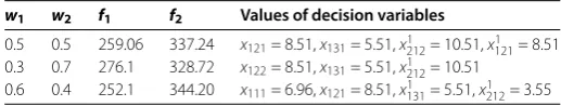
Table 5 Optimum results by using the convex combination method for Model-2

w1 w2 f1 f2 Values of decision variables

0.5 0.5 259.06 337.24 x121= 8.51,x131= 5.51,x1212= 10.51,x1121= 8.51

0.3 0.7 276.1 328.72 x122= 8.51,x131= 5.51,x1212= 10.51

Table 6 Comparison of optimum results of Model-2

Method f1 f2 Values of decision variables

FISM 273.40 330.07 x121= 1.34,x122= 7.16,x131= 5.51,x212= 10.51

Convex combination 252.1 344.20 x111= 6.96,x121= 8.51,x131= 5.51,x212= 3.55

Global criteria 259.06 337.24 x121= 8.51,x131= 5.51,x212= 10.51,GC= 0.0514

7.3 Optimum result for Model-3

To solve Model-, we will solve MSSTPα (Example .) and the optimum solution has

come for decisionα∗= ., and the optimal solutions for different items are

⎡ ⎢ ⎢ ⎢ ⎣

x()_ x()_ x()_ x()_ x()_ x()_ x() x

()

 x

()  x()_ x()_ x()_

⎤ ⎥ ⎥ ⎥ ⎦=

⎡ ⎢ ⎢ ⎢ ⎣

 . 

  .

.  

 .  ⎤ ⎥ ⎥ ⎥ ⎦,

⎡ ⎢ ⎢ ⎢ ⎣

x()_ x()_ x()_ x()_ x()_ x()_ x()_ x()_ x()_ x()_ x()_ x()_

⎤ ⎥ ⎥ ⎥ ⎦=

⎡ ⎢ ⎢ ⎢ ⎣

 . .

.  

 . 

  .

⎤ ⎥ ⎥ ⎥ ⎦

and the corresponding optimal values for different items are

f_() f_() f_() f_()

=

 . . .

.

8 Conclusion

The multi-objective multi-item solid transportation problem in fuzzy inequality con-straints has been explored in this paper. Three different models have been derived. First, a fuzzy inequality solid transportation problem has been converted to a parametric solid transportation problem using flexible index, and then the fuzzy inequality solid trans-portation problem has been solved by using the decision making technique. The fuzzy interactive satisfied method, global criterion method and convex combination method have been applied to calculate the optimal compromise solutions of multi-objective STP problem, and then it was solved by using MatLab and Lingo-.. The models are illus-trated with numerical examples and corresponding results are compared. This paper only researches the problem under fuzzy inequality constraints, and the problem in other more complex environments or multi-objective uncertain transportation problem may become new topics in further research. The present formulation and solution procedures can be applied to other fuzzy transportation models with different fuzzy numbers.

Appendix

Example . Consider the following FICP:

minx_+ x_+ x_+ x_ + x_+ x_ + x_+ x_

+ x_+ x_+ x_+ x_+ x_+ x_+ x_+ x_

s.t.x_+x_+x_+x_+x_+x_,

x_+x_+x_+x_+x_+x_,

x_+x_+x_+x_,

x_+x_+x_+x_,

x_+x_+x_+x_,

x_+x_+x_+x_+x_+x_,

x_+x_+x_+x_+x_+x_,

x_+x_+x_+x_,

MMSTP x_+x_+x_+x_,

x_+x_+x_+x_,

x_+x_+x_+x_+x_+x_+x_

+x_+x_+x_ +x_+x_,

x_+x_+x_+x_+x_+x_+x_

+x_+x_+x_ +x_+x_,

xp_ijk≥ ∀i,j,kandp= , , d= (, , , , , , , , , , , ).

The corresponding parametric linear programming problem ofMMSTP is presented as follows:

minx_+ x_+ x_ + x_+ x_+ x_

+ x_+ x_+ x_+ x_+ x_+ x_

+ x_+ x_+ x_+ x_+ x_+ x_

+ x_+ x_+ x_+ x_+ x_+ x_

s.t.x_+x_+x_+x_+x_+x_≤,

x_+x_+x_+x_+x_+x_≤,

x_+x_+x_+x_≥,

x_+x_+x_+x_≥,

x_+x_+x_+x_≥,

x_+x_+x_+x_+x_+x_≤, ()

x_+x_+x_+x_+x_+x_≤ + ( –a),

x_+x_+x_+x_≥ + ( –α),

MMSTPα x_+x_+x_+x_≥ + ( –α),

x_+x_+x_+x_≥ + ( –α),

+x_+x_+x_+x_+x_≤ + ( –α),

x_+x_+x_+x_+x_+x_+x_

+x_+x_+x_+x_+x_≤ + ( –α),

xp_ijk≥ ∀i,j,k,p= ,  and ≤α≤.

Now, using the algorithm given in Section ., we obtainZ= ,Z=  andd=  by calculating (MMSTP) and (MMSTP) corresponding to (). Let the inverse of the optimal matrix in (MMSTP) be

B–_ = ⎛ ⎜ ⎜ ⎜ ⎜ ⎜ ⎜ ⎜ ⎜ ⎜ ⎜ ⎜ ⎜ ⎜ ⎜ ⎜ ⎜ ⎜ ⎜ ⎜ ⎜ ⎜ ⎜ ⎜ ⎝

       –  –  –

           

    –   –  –  –

   –        

           

           

           

       –    

        –   

         –  

           

  –         

⎞ ⎟ ⎟ ⎟ ⎟ ⎟ ⎟ ⎟ ⎟ ⎟ ⎟ ⎟ ⎟ ⎟ ⎟ ⎟ ⎟ ⎟ ⎟ ⎟ ⎟ ⎟ ⎟ ⎟ ⎠ .

Now, calculating the equations [B–

(, , , , , ,  + ( –α),  + ( –α),  + ( –

α),  + ( –α),  + ( –α),  + ( –α))]i=  (i= , , . . . , ), respectively, we obtain

α= . assumeα=  andα= .

Now, solving (MMSTPα), we get an optimal solution and an optimal value as Zα= Z.= ..

Now,Z.= . <Z+ .× = ., so we stop here and calculate optimal decisionα∗. Now

α∗=Zα–Zα–Zαα+Zαα Zα–Zα–αd+αd

= ..

Now, solving (MMSTP.), we obtain the optimal valueZ∗_.= ..

Example . Consider the following FICP:

minx+ x+ x+ x

+ x+ x+ x+ x

+ x+ x+ x+ x

s.t.x+x+x+x+x+x,

x+x+x+x, ()

x+x+x+x,

MSSTP x+x+x+x,

x+x+x +x+x+x,

x+x+x+x+x+x,

xijk≥ ∀i,j,k, d= (, , , , , , ).

The corresponding parametric linear programming problem ofMSSTP is presented as follows:

minx+ x+ x+ x

+ x+ x+ x+ x

+ x+ x+ x+ x

s.t.x+x+x+x+x+x≤,

x+x+x+x+x+x≤,

x+x+x+x≥ + ( –α), ()

x+x+x+x + ( –α),

MSSTPα x+x+x+x≥ + ( –α),

x+x+x +x+x+x≤ + ( –α),

x+x+x+x+x+x≤ + ( –α),

xijk≥ ∀i,j,k, ≤α≤.

Now, using the algorithm given in Section ., we obtainZ= ,Z=  andd=  by calculating (MSSTP) and (MSSTP) corresponding to (). The inverse of the optimal matrix in (MSSTP) is

B–_ = ⎛ ⎜ ⎜ ⎜ ⎜ ⎜ ⎜ ⎜ ⎜ ⎜ ⎜ ⎜ ⎝

–  – – –  

      

      

   –   

    –  

–      

      

⎞ ⎟ ⎟ ⎟ ⎟ ⎟ ⎟ ⎟ ⎟ ⎟ ⎟ ⎟ ⎠ .

Now, calculating the equations [B–

(, ,  + ( –α),  + ( –α),  + ( –α),  + ( –

α),  + ( –α))]i=  (i= , , . . . , ), respectively, we obtainα= . assumeα= 

andα= .

Now, solving (MSSTPα), we get an optimal solution asx= ,x=  andx=  and

NowZ.= . <Z+ .× = ., so we stop here and calculate opti-mal decisionα∗. Now

α∗=Zα–Zα–Zαα+Zαα Zα–Zα–αd+αd

= ..

Now, solving (MSSTP.), we obtain an optimal value asZ∗_{.}= ..

Competing interests

The authors declare that they have no competing interests.

Authors’ contributions

All authors contributed equally to the writing of this paper. All authors read and approved the final manuscript.

Author details

1_{Department of Mathematics, Heritage Institute of Technology, Anandapur, Kolkata, West Bengal 700107, India.} 2_{Department of Applied Science, Haldia Institute of Technology, Purba Midnapur, Haldia, West Bengal 721657, India.} 3_{Department of Mathematics, Bengal Engineering and Science University, Shibpur, Howrah, West Bengal 711103, India.}

Acknowledgements

The authors sincerely thank the anonymous reviewers and editor-in-chief for their careful reading, constructive comments and fruitful suggestions. The first two authors are also thankful to Ms. Priyanka Dey, Assistant Professor, Haldia Institute of Technology for advices on grammatical errors and organization of the paper.

Received: 23 April 2014 Accepted: 19 August 2014 Published:03 Sep 2014

References

1. Haley, K: The solid transportation problem. Oper. Res.10, 448-463 (1962)

2. Ojha, A, Das, B, Mondal, S, Maiti, M: A solid transportation problem for an item with fixed charge, vehicle cost and price discounted varying charge using genetic algorithm. Appl. Soft Comput.10, 100-110 (2010)

3. Pramanik, S, Jana, DK, Maiti, K: A multi objective solid transportation problem in fuzzy, bi-fuzzy environment via genetic algorithm. Int. J. Adv. Oper. Manag.6(1), 4-26 (2014)

4. Bit, AK, Biswal, MP, Alam, SS: Fuzzy programming approach to multi-objective solid transportation problem. Fuzzy Sets Syst.57, 183-194 (1993)

5. Ida, K, Gen, M, Li, Y: Neural networks for solving multicriteria solid transportation problem. Comput. Ind. Eng.31, 873-877 (1996)

6. Gao, SP, Liu, SY: Two-phase fuzzy algorithms for multi-objective transportation problem. J. Fuzzy Math.12, 147-155 (2004)

7. Tao, Z, Xu, J: A class of rough multiple objective programming and its application to solid transportation problem. Inf. Sci.188, 215-235 (2012)

8. Kundu, P, Kar, S, Maiti, M: Multi-objective multi-item solid transportation problem in fuzzy environment. Appl. Math. Model.37, 2028-2038 (2013)

9. Pramanik, S, Jana, DK, Maiti, M: Multi-objective solid transportation problem in imprecise environment. J. Transp. Secur.6, 131-150 (2013)

10. Sancak, E, Salman, S: Multi-item dynamic lot-sizing with delayed transportation policy. Int. J. Prod. Econ.131, 595-603 (2011)

11. Zimmermann, HJ: Fuzzy programming and linear programming with several objective functions. Fuzzy Sets Syst.1, 45-55 (1978)

12. Zimmermann, HJ: Description and optimization of fuzzy systems. Int. J. Gen. Syst.2, 209-215 (1976) 13. Cao, BY: Optimal Models and Methods with Fuzzy Quantities. Springer, Berlin (2010)

14. Sakawa, K: Fuzzy Sets and Interactive Multiobjective Optimization. Plenum, New York (1993) 15. Xu, J, Zhou, X: Fuzzy Like Multiple Objective Decision Making. Springer, Berlin (2011)

10.1186/1029-242X-2014-338