2018 International Conference on Computer, Communication and Network Technology (CCNT 2018) ISBN: 978-1-60595-561-2
An Artificial Intelligence (AI) Defect Detection Technology Based on
Software Behavior Decision Tree
Xiang-zhou CHEN
1, Hui-xia DING
1,*, Jie ZHANG
2, Yang WANG
1,
Geng ZHANG
1and Ya-nan WANG
11
Information & Communication Department CEPRI, China 2
North China Electric Power University, China
*Corresponding author
Keywords: Artificial intelligence (AI) defect detection, Machine learning, Decision tree, Layered detection, Software test.
Abstract. With the increase of software system complexity, a high requirement of the reliability, stability and security of software quality is put forward. At present, artificial intelligence (AI) defect detection adoptes machine learning technology to realize code scanning and semantic analysis on software defects. The traditional machine learning technology for software defect detection is generally based on algorithms such as BP neural network model, Naïve-Bayes model, and fingerprint identification model, etc. Regarding the features of software artificial intelligence (AI) defect detection, this paper proposes a layered detection technology based on software behavior decision tree model. Furthermore, a corresponding test environment is established to make contrast test of previously tested software. The results of the experiment shows that, with the comprehensive consideration of building time cost and false alarm rate and other factors, the artificial intelligence (AI) defect detection technology based on software behavior decision tree model is superior to other technologies.
Introduction
At present, with the rise of the demand of Internet application, the rapid growth of software size and the increase of hierarchy and complexity of system architecture, the types and quantities of software defects become the determinants of software reliability, maintainability, portability, usability and efficiency. Software artificial intelligence (AI) defect detection refers to using the historical data that is formed during the process of software test, to construct a prediction model in an abstract way, and finally, to achieve defect analysis of a certain software. Software artificial intelligence (AI) defect detection can improve the reliability of software quality during its development, and reduce maintenance cost during its upgrade and maintenance. Meanwhile, the decrease of software defects can effectively reduce the workload in the cross-platform migration process, improve the user experience, and finally realize the efficient operation.
Another type of artificial intelligence (AI) defect detection method is called dynamic detection method, which mainly refers to the detection during software operation, and the method of engineering is used to measure and control the state of software operation. The detection methods mainly include: non-execution stack, non-execution heap and data, memory mapping, secure Shared library, sandbox and program interpretation, etc. This kind of method belongs to active detection measure. The research of dynamic detection methods was once limited by the performance of computer and was limited within the theoretical research stage, however, with the continuous improvement of computer performance, some mature dynamic detection technology, dynamic detection without changing the source code or even under the condition of binary code, to detect the application weaknesses, mainly by modifying the process’s operation environment.
Introduction to Software Behavior Modeling Technology
Software behavior refers to the actions or actions imposed by the software that is running on the computer system. The execution of software behavior consists of the control flow and the data stream. The research contents of construction of software behavior model include: characteristic, state, mode and structure. The focuses of the study are as follows: behavior structure relationship, the relationship between main structure of individual behavior and group behavior, the relationship between the hierarchical structure of behavior and group behavior, the expansion of the new ability of software cluster behavior model compared with the individual behavior model.
Software behavior model also studies the behavior of subject to object, the behavior of subject to subject as well as the behavior of subject to system. Furthermore, it studies the influence of software behavior model on computer or system security, as well as the influence of software behavior on other software behaviors. Software behavior modeling technology consists of: short sequence, machine learning, automaton, static modeling, etc.
Short Sequences
Machine Learning
Based on machine learning modeling method, the normal behavior mode of program can be concluded by means of machine learning technology. The short sequence model introduced in the last section is especially suitable for the optimization with some techniques from artificial intelligence, so the machine learning model is essentially the optimization and improvement based on the short sequence model. Yin [5] uses the state sequence output from output of the hidden Markov model to determine whether abnormal behavior occurs. The hidden Markov model has the characteristics of high precision and complicated calculation. Bouguila et al. [6] uses Bayesian network to construct statistical model to analyze and predict the future behavior of the program. Ghosh, Endler et al. [7] introduces artificial neural network to realize behavior detection. The performance of neural network model is solid, but the computational complexity increases with the number of neurons, which brings difficulty to the search of suitable network. Liao [8] adopts the text classification technique, which regards software behavior as a document, records the occurrence frequency of different system call in the document and presents them vectorially, the classifier is employed to determine the untested behaviors. However, the method only considers the frequency characteristics of system calls, it lacks completeness. Lee [9] proposes a sequence pattern which extracts system call sequences using data mining technology. Firstly, a correlation analysis is made on similar short sequences, then several representative sequence patterns are quoted to represent these short sequences, finally, the Ripper algorithm is employed to establish the rule library. This model can effectively reduce storage overhead and improve detection efficiency and simplify the modeling complexity. In order to further simplify the complexity of modeling, Cai et al. [10] introduces the rough set theory during the process of sequential mode mining. In addition, Zhang classifies system calls by effect, and only records the system calls with significant security concerns, which greatly reduces the storage overhead and computation time. Look-ahead pairs uses a structure similar to regular expression to describe local patterns in a compact and efficient way. As can be seen from the above introduction, most machine learning models are optimization and simplifications of sequential patterns. Among these methods, their accuracy is almost on the same level, except for the model based on hidden Markov, whose accuracy level is comparatively higher. Since the system call sequence has a strong regularity itself, simple models are able to work effectively, on the contrary, machine learning models are often limited by the technology itself, it is hard to improve their accuracy without technological development.
Automaton
Sekar [11] establishes the FSA model dynamically with the help of system call and its PC value. The model can effectively track the loop, branch, jump and other information, but there is a problem of “impossible path”. In order to to solve the problem, puts forward the Vt Path model, combining the call stack information and the program counter value dynamically the model builds virtual stack tables. With the help of virtual stack, current system calls and the virtual paths between system calls are calculated, which improves the accuracy and efficiency of the model. But since two hash tables are required to construct a model, the space complexity is also higher. Subsequently, Feng puts forward a static version of the Vt Path model, the VP static model. Static-dynamic combined methods are employed in most of the following automatons in order to retain the advantages of both dynamic and static modeling, The Dyck model proposed by Giffin first establishes the model by static analysis of binary code, and then the model is simplified through dynamic analysis. The model takes system call parameters, previous and following context and other factors into overall consideration, to achieve a high accuracy.
Static Modeling
widely cited, which belongs to the static model of automaton. The call graph is actually a non-deterministic Finite Automata (NFA). It defines the state nodes in the graph using the function call location in the source code. The call graph model is simple and practical, but impossible execution paths are found in it in actual situations. Therefore, Wagner extends the call graph model, adds a push stack to save the return location corresponding to the function calls. In this way, an undetermined push-down automaton and the corresponding context-free grammar are obtained, which is called “abstract stack model”. Although the problem of impossible path is solved, the operation cost is extremely high, which seriously affects the real-time performance of the detection system.
Decision Tree Detection Technology
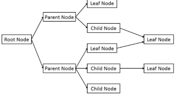
[image:4.612.164.453.271.431.2]Decision tree learning is an example based induction learning algorithm. It is a simple and effective fast classification algorithm commonly used in data mining. It focuses on the classification rules represented by decision trees in a set of unordered, rule-based examples. The decision tree model diagram is shown in Figure 1:
Figure 1. Decision tree model.
The most commonly used algorithm of decision tree classification model is the C4.5 algorithm, a decision tree learning algorithm based on information entropy. The C4.5 algorithm is based on the advantages of ID3 and some improvements are made for the purpose of achieving a data mining efficiency over the ID3 algorithm. Instead of using information gain, the information gain rate is adopted as the standard. This is a refinement of information gain to remove the effects of high branch properties. The method of information gain takes the number of child nodes you generate and the size of each child node (including the number of data instances) of each time into consideration simultaneously. The object of consideration is the division of one by one, rather than the amount of information contained in the classification.
The formula is:
2
=
1
Gain(A) Gain Ratio (A)
Split I(S , S ... Sv) (1)
( 1, 2... ) ( ) Split I S S Sv pjlb p
j
=∑
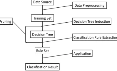
(2) Where v is the number of branches of the node, Sv is the number of records under subdivision v. The Figure 2 mainly introduces the process of initializing a decision tree via the training set obtained through data preprocessing and the summary of data set.
When training for the training set. Calculate the information Gain (A) and Gain Ratio (A) of each attribute. Choose the attributes with the largest information gain which is no lower than the average value of all attributes. The current main attribute node execute recursively the above for the samples in its child node, until the data records in the subset being the same as the values of main attributes, or no attribute being divisible. Initialize the decision tree.
[image:5.612.214.413.151.272.2]Software behavior artificial intelligence (AI) defect detection technology under decision tree model.
Figure 2. Decision tree classification model.
According to the definition of decision tree model, together with software defects, the following definitions are made: software behavior set B, riskless normal behavior set S, potential risk behavior set P, abnormal behavior set A,
According to the definition,
{ , , } B= S P A
(3)
S∩P=P∩A=S∩A= Φ (4)
Firstly, software behavior is divided into 3 big categories and 8 small categories:
1) Riskless normal behaviors S: normally executes corresponding instructions, without illegal call to system resources, without the problem of normal software operation ability damage or normal behavior error, not on the system and the behavior of functional and nonfunctional into effect. And this behavior does not affect the function and non-function of the related system.
2) Potential risk behaviors P: the corresponding instruction is basically executed, with the risk of reducing system performance and the increase of potential risk:
a) Function defect behaviors: the behavior instruction causes inconsistencies between the function realized by the program and the behavior’s request, leading to unexpected behaviors.
b) System defect behaviors: due to the interconnection between the subsystem and module within the program, the behaviors and the defects related to the operating system result in errors.
c) Unauthorized behaviors: due to the loopholes in security policy control, roles permissions and management control, unauthorized behavior by unauthenticated users through this kind of loopholes, can lead to data breaches, malicious changes, access uncontrol and other consequences.
3) Abnormal behavior A:
a) Data abnormal behaviors: the behavior leads to unauthenticated users’ data manipulations in the database, unpunctual and ineffective access to the database system and its data offers, and unauthenticated users’ accessibility to data in the database.
b) Operation abnormal behaviors: abnormal input, output or method parameter errors lead to slow responses during the software operation, abnormal IO throughputs, excessive resource occupations and other behaviors.
d) Information interaction behaviors: the existence of these behaviors result in business exceptions, such as the possibility of abnormal negative inventory and inventory data bits empty anomalies. Besides, this kind of behavior can throw IP exceptions between clients and servers, leading to unstable communication between interfaces.
[image:6.612.196.427.151.295.2]The flowchart of a decision tree model for software behavior artificial intelligence (AI) defect detection is shown in Figure 3:
Figure 3. Software behavior artificial intelligence (AI) defect detection.
Prototype Design and Implementation of Defect Detection Platform Based on Software Behavior Decision Tree
The Multi-viewpoint Three-layer Modeling Technology for Information System
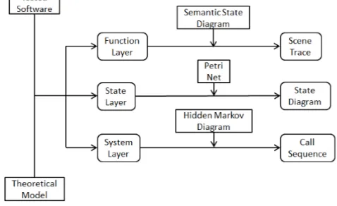
At present, the research of software behavior model focuses on software operation path analysis, which lacks adequate consideration of system call parameters and software operation’s background environment information. However, the behavior model considering various behavioral characteristics is not optimal in terms of detection efficiency because of its high complexity. The analysis of software behavior usually only focuses on the control flow or data flow of the system, and the artificial intelligence (AI) defect detection rate is not satisfactory. In response to the above problems, the layered modeling of the three-layer system (system layer, state layer and function layer) is implemented based on the multi-view modeling method. The Figure 4 shows a typical artificial intelligence (AI) defect detection platform based on three-layer modeling:
Figure 4. Artificial intelligence (AI) defect detection platform.
[image:6.612.192.431.521.667.2]accurately. The implementation of software behavior artificial intelligence (AI) defect detection is one of the key points and difficulties of this project.
Function Logic Artificial Intelligence (AI) Defect Detection and Analysis Technology Based on Mixed Strategy
[image:7.612.165.463.230.330.2]The detection and analysis of software behavior can also be used in different layers, in the state layer and the system layer, and the status sequence is tested according to deviation density. If there is an exception, an alarm directly occurs, if not, the test turns to the next step. The second step is to detect the function layer, and to distinguish the software function sequence based on the functional semantic rules. All violations of the rules are determined as abnormal. Then the detection capability of the model is analyzed from the angle of attacker. The Figure 5 gives an example of the flow-process of a function logic artificial intelligence (AI) defect detection:
Figure 5. Function logic artificial intelligence (AI) defect detection.
According to the model definition, on the cloud test platform, the deviation density trajectory tracking and analysis technique is used to excavate the relationship between the software’s behavior process and effect. Then the relationship is refined into a behavior template and stored in a knowledge base. The behavior trace information of the running system is then compared with the behavior template to detect potential defects.
Application Result and Analysis of Artificial Intelligence (AI) Defect Detection Technology
Test Application Results of Business Information System
For the existing business system, 61 business information systems are randomly selected and divided into two groups:
Control group: functional test adopts QTP combined with artificial detection as retest, performance test adopts Loadrunner as the pressure test tool, and security test adopts Fortify SCA as the basic detection tool, with auxiliary artificial verification.
Experimental group: functional tests adopts QTP combined with prototype test, performance test adopts Loadrunner as the pressure test tool, and security test adopts the prototype test as the basic test tool, with auxiliary artificial inspections. The results are as follows:
1) Control group
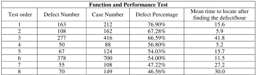
Table 1. Function and performance test 1.
Function and Performance Test
Test order Defect Number Case Number Defect Percentage Mean time to locate after finding the defect/hour
1 163 212 76.90% 15.6
2 108 162 67.28% 5.9
3 277 416 66.59% 41.8
4 50 88 56.80% 5.2
5 67 124 54.03% 15.7
6 378 700 54.00% 11.5
7 55 108 47.22% 27.2
[image:7.612.98.514.623.745.2]Function and Performance Test
Test order Defect Number Case Number Defect Percentage Mean time to locate after finding the defect/hour
9 46 100 46.00% 1.5
10 43 109 43.25% 36.0
11 467 1016 41.00% 7.4
12 61 155 39.35% 12.0
13 79 251 37.97% 41.1
14 41 454 37.86% 44.1
15 89 237 37.55% 43.6
16 88 186 34.07% 39.2
17 64 190 33.68% 2.0
18 168 504 33.00% 38.6
19 70 213 32.86% 38.0
20 49 162 30.25% 16.5
21 106 351 30.20% 44.7
22 17 57 29.82% 21.4
23 107 359 29.81% 40.1
24 48 135 29.00% 20.6
25 118 407 28.99% 4.5
26 148 38 25.68% 3.3
27 55 218 25.20% 12.7
28 66 260 25.00% 16.2
29 37 148 25% 31.8
30 32 136 22.79% 24.9
31 77 351 21.94% 34.2
32 61 286 21.30% 42.4
33 32 150 21.30% 35.9
34 143 714 20.03% 46.1
35 34 180 18.89% 47.1
36 84 445 18.88% 47.2
37 48 259 18.53% 15.6
38 42 569 18.42% 33.5
39 42 228 18.42% 30.9
40 44 239 18.40% 18.2
41 21 115 18.26% 43.0
42 18 106 17.90% 24.2
43 122 707 17.26% 25.2
44 57 336 16.97% 34.7
45 56 56 15.18% 13.4
46 44 295 14.92% 14.2
47 32 215 14.88% 31.6
48 51 356 14.33% 47.8
49 41 313 13.10% 0.1
50 176 23 13.06% 23.9
51 338 3017 12.72% 9.6
52 63 496 12.70% 10.5
53 113 1214 12.39% 6.6
54 90 746 12.06% 16.6
55 8 78 10.26% 22.7
56 8 78 10.26% 13.3
57 28 259 10.00% 0.1
58 8 81 10% 27.1
59 8 85 9.41% 5.9
60 4 49 8.16% 33.1
61 16 360 4.44% 11.9
Table 2. Security test 1.
Security Test
Test order Defect Number Case Number Defect Percentage Mean time to locate after finding the defect/hour
Security Test
Test order Defect Number Case Number Defect Percentage Mean time to locate after finding the defect/hour
2 23 71 32.39% 3.7
3 21 71 29.58% 10.3
4 11 71 15.49% 19.9
5 22 71 30.99% 39.4
6 23 71 32.39% 30.6
7 21 71 29.58% 33.1
8 14 71 19.72% 39.4
9 17 71 23.94% 28.9
10 32 71 45.07% 23.8
11 17 71 23.94% 7.1
12 55 71 77.46% 20.8
13 8 71 11.27% 15.6
14 10 71 14.08% 48.2
15 18 71 25.35% 9.5
16 15 71 21.13% 44.8
17 18 71 25.35% 46.1
18 36 71 50.70% 34.5
19 21 71 29.58% 16.9
20 15 71 21.13% 43.3
21 38 71 53.52% 42.7
22 14 71 19.72% 16.0
23 11 71 15.49% 34.2
24 9 71 12.68% 24.6
25 14 71 19.72% 2.9
26 22 71 30.99% 26.2
27 10 71 14.08% 28.1
28 27 71 38.03% 16.8
29 61 71 85.92% 33.6
30 52 71 73.24% 43.9
31 28 71 39.44% 36.3
32 6 71 8.45% 0.9
33 29 71 40.85% 15.2
34 20 71 28.17% 50.0
35 46 71 64.79% 18.7
36 28 71 39.44% 29.2
37 26 71 36.62% 45.7
38 8 71 11.27% 1.5
39 11 71 15.49% 14.0
40 37 71 52.11% 1.7
41 25 71 35.21% 8.5
42 16 71 22.54% 32.1
43 13 71 18.31% 29.4
44 38 71 53.52% 14.7
45 41 71 57.75% 39.4
46 10 71 14.08% 44.0
47 3 71 4.23% 22.9
48 10 71 14.08% 4.0
49 17 71 23.94% 32.9
50 20 71 28.17% 25.2
51 5 71 7.04% 15.9
52 19 71 26.76% 1.0
53 34 71 47.89% 33.6
54 21 71 29.58% 4.5
55 9 71 12.68% 36.4
56 46 71 64.79% 25.4
57 23 71 32.39% 9.1
58 21 71 29.58% 39.0
59 11 71 15.49% 17.2
Security Test
Test order Defect Number Case Number Defect Percentage Mean time to locate after finding the defect/hour
61 23 71 32.39% 12.4
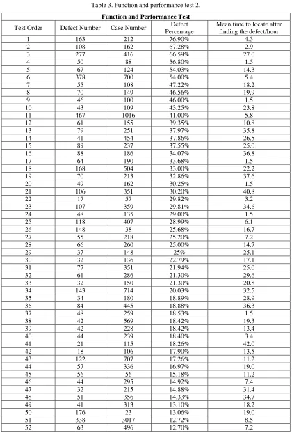
[image:10.612.96.516.129.751.2]2) Experimental group
Table 3. Function and performance test 2.
Function and Performance Test
Test Order Defect Number Case Number Defect Percentage
Mean time to locate after finding the defect/hour
1 163 212 76.90% 4.3
2 108 162 67.28% 2.9
3 277 416 66.59% 27.0
4 50 88 56.80% 1.5
5 67 124 54.03% 14.3
6 378 700 54.00% 5.4
7 55 108 47.22% 18.2
8 70 149 46.56% 19.9
9 46 100 46.00% 1.5
10 43 109 43.25% 23.8
11 467 1016 41.00% 5.8
12 61 155 39.35% 10.8
13 79 251 37.97% 35.8
14 41 454 37.86% 26.5
15 89 237 37.55% 25.0
16 88 186 34.07% 36.8
17 64 190 33.68% 1.5
18 168 504 33.00% 22.2
19 70 213 32.86% 37.6
20 49 162 30.25% 1.5
21 106 351 30.20% 40.8
22 17 57 29.82% 3.2
23 107 359 29.81% 34.6
24 48 135 29.00% 1.5
25 118 407 28.99% 6.1
26 148 38 25.68% 16.7
27 55 218 25.20% 7.2
28 66 260 25.00% 14.7
29 37 148 25% 25.1
30 32 136 22.79% 17.1
31 77 351 21.94% 25.0
32 61 286 21.30% 29.6
33 32 150 21.30% 20.8
34 143 714 20.03% 32.5
35 34 180 18.89% 28.9
36 84 445 18.88% 36.3
37 48 259 18.53% 1.5
38 42 569 18.42% 19.3
39 42 228 18.42% 13.4
40 44 239 18.40% 3.4
41 21 115 18.26% 42.0
42 18 106 17.90% 13.5
43 122 707 17.26% 11.2
44 57 336 16.97% 19.0
45 56 56 15.18% 11.2
46 44 295 14.92% 7.4
47 32 215 14.88% 31.4
48 51 356 14.33% 34.7
49 41 313 13.10% 18.2
50 176 23 13.06% 19.0
51 338 3017 12.72% 8.5
Function and Performance Test
Test Order Defect Number Case Number Defect Percentage
Mean time to locate after finding the defect/hour
53 113 1214 12.39% 5.0
54 90 746 12.06% 3.2
55 8 78 10.26% 22.6
56 8 78 10.26% 1.0
57 28 259 10.00% 3.5
58 8 81 10% 23.0
59 8 85 9.41% 7.6
60 4 49 8.16% 22.0
[image:11.612.98.516.61.753.2]61 16 360 4.44% 9.2
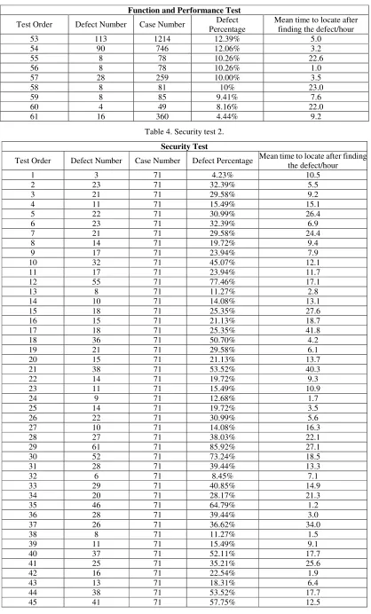
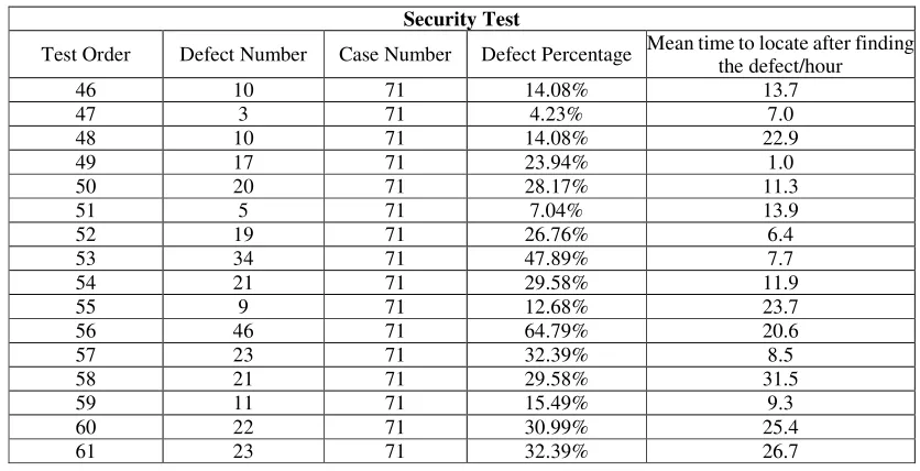
Table 4. Security test 2.
Security Test
Test Order Defect Number Case Number Defect Percentage Mean time to locate after finding the defect/hour
1 3 71 4.23% 10.5
2 23 71 32.39% 5.5
3 21 71 29.58% 9.2
4 11 71 15.49% 15.1
5 22 71 30.99% 26.4
6 23 71 32.39% 6.9
7 21 71 29.58% 24.4
8 14 71 19.72% 9.4
9 17 71 23.94% 7.9
10 32 71 45.07% 12.1
11 17 71 23.94% 11.7
12 55 71 77.46% 17.1
13 8 71 11.27% 2.8
14 10 71 14.08% 13.1
15 18 71 25.35% 27.6
16 15 71 21.13% 18.7
17 18 71 25.35% 41.8
18 36 71 50.70% 4.2
19 21 71 29.58% 6.1
20 15 71 21.13% 13.7
21 38 71 53.52% 40.3
22 14 71 19.72% 9.3
23 11 71 15.49% 10.9
24 9 71 12.68% 1.7
25 14 71 19.72% 3.5
26 22 71 30.99% 5.6
27 10 71 14.08% 16.3
28 27 71 38.03% 22.1
29 61 71 85.92% 27.1
30 52 71 73.24% 18.5
31 28 71 39.44% 13.3
32 6 71 8.45% 7.1
33 29 71 40.85% 14.9
34 20 71 28.17% 21.3
35 46 71 64.79% 1.2
36 28 71 39.44% 3.0
37 26 71 36.62% 34.0
38 8 71 11.27% 1.5
39 11 71 15.49% 9.1
40 37 71 52.11% 17.7
41 25 71 35.21% 25.6
42 16 71 22.54% 1.9
43 13 71 18.31% 6.4
44 38 71 53.52% 17.7
Security Test
Test Order Defect Number Case Number Defect Percentage Mean time to locate after finding the defect/hour
46 10 71 14.08% 13.7
47 3 71 4.23% 7.0
48 10 71 14.08% 22.9
49 17 71 23.94% 1.0
50 20 71 28.17% 11.3
51 5 71 7.04% 13.9
52 19 71 26.76% 6.4
53 34 71 47.89% 7.7
54 21 71 29.58% 11.9
55 9 71 12.68% 23.7
56 46 71 64.79% 20.6
57 23 71 32.39% 8.5
58 21 71 29.58% 31.5
59 11 71 15.49% 9.3
60 22 71 30.99% 25.4
61 23 71 32.39% 26.7
Result Analysis
[image:12.612.96.514.65.279.2]Through a random sample of electric power information system has been developed to complete the test, the decision tree based on software behavior of artificial intelligence (AI) defect detection platform prototype artificial intelligence (AI) defect detection of function and performance have obvious effect, concrete results in Figure 6:
Figure 6. Mean locating time after found function and performance defects.
[image:12.612.192.425.366.430.2]Following the security defect test, the specific results are analyzed in Figure 7:
Figure 7. Mean locating time after found security defects.
After comparison, it is found that the prototype of the artificial intelligence (AI) defect detection platform based on the software behavior decision tree has obvious effect on the function and performance artificial intelligence (AI) defect detection, which increase the defect location efficiency by 47.38%. Meanwhile, on the security test, an average increase of 11.94% of defect location efficiency is found.
Cause Analysis
corresponding system module immediately according to the corresponding exceptions. Therefore, this test system is more sensitive to function tests.
2) Security test mainly includes user access control strategy, network access control, audit strategy, data transmission confidentiality and penetration test, the test cases have a total of 71 items. In addition, except for the audit strategy and data transmission confidentiality which involve less code modules, the other three directions are all closely related to functional modules, hence there is a certain degree of deviation in the process of locating.
3) In the detection of the system layer, a security penetration defect or a clear text transmission loopholes does not cause a system malfunction easily. But when the invaders implement session replay attacks, replay attacks and other forms of security attacks, the corresponding defects can be tested out. Therefore, under the existing test environment, the code base requires continuous upgrades.
Summary
Software artificial intelligence (AI) defect detection is an important research direction in the field of software test, this paper puts forward a hierarchical detection technology based on software behavior decision tree model and sets up a corresponding test platform. Through the contrast experiment on the previously developed software, it is found that the model is relatively sensitive to defects of software function and performance, and in contrast, less sensitive to security loopholes. In the later study, addition of semantic analysis and research concerning the vulnerability database requires to be taken into consideration. At the same time, there remains some further researches to be done on feature extractions and defect classifications.
Acknowledgement
This work is supported by the State Grid Scientific Project which names Research on Comprehensive Simulation and Quality Evaluation of Power Communication Network (No. XX71-16-004).
References
[1]Kymie M, C Tan, “The Application of Neural Networks to UNIX Computer Security”, Proceedings of the IEEE International Conference on Neural Networks, 1993.
[2]Debar H, et al, “Fixed vs. variable-Length Patterns for Detecting Suspicious Process Behavior”, 5th European Symposium on Research in Computer Security (ESORICS ’98), 1998.
[3]H. Debar, A. Wespi, “Aggregation and correlation of intrusion-detection alerts”, Recent Advances in Intrusion Detection (RAID 2001), 2001.
[4]Lihong Yao, et al, “Bing Research of System Call Based Intrusion Detection”, ACTA electronic ASINICA, 2003.
[5]G Yin, Q Zhang, “Continuous-time Markov chains and applications”, Applications of Mathematics, 1998.
[6]Nizar Bouguila, “Bayesian hybrid generative discriminative learning based on finite Liouville mixture models[J]”, Pattern Recognition, 2010.
[7]A.K. Ghosh, J. Wanken, and F. Charron, “Detecting anomalous and unknown intrusions against programs”, ACSAC '98 Proceedings of the 14th Annual Computer Security Applications Conference, 1998.
[9]Wenke Lee, Dong Xiang, “Information-Theoretic measures for anomaly detection”, IEEE Symposium on Security & Privacy, 2001.
[10]Jiawei Han, Yandong Cai et al, “Data-driven discovery of quantitative rule in relation database”, IEEE Transactions on Knowledge and Data Engineering, 1993.