Fluid queues driven by a discouraged arrivals queue

PII. S0161171203203203 http://ijmms.hindawi.com © Hindawi Publishing Corp.

FLUID QUEUES DRIVEN BY A DISCOURAGED

ARRIVALS QUEUE

P. R. PARTHASARATHY and K. V. VIJAYASHREE

Received 20 March 2002

We consider a fluid queue driven by a discouraged arrivals queue and obtain ex-plicit expressions for the stationary distribution function of the buffer content in terms of confluent hypergeometric functions. We compare it with a fluid queue driven by an infinite server queue. Numerical results are presented to compare the behaviour of the buffer content distributions for both these models.

2000 Mathematics Subject Classification: 60K25.

1. Introduction. Stochastic fluid flow models are increasingly used in the performance analysis of communication and manufacturing models. Recent measurements have revealed that in high-speed telecommunication networks, like the ATM-based broadband ISDN, traffic conditions exhibit long-range de-pendence and burstiness over a wide range of time scales. Fluid models char-acterize such traffic as a continuous stream with a parameterized flow rate.

Fluid queue models, where the fluid rates are controlled by state-dependent rates, have been studied in the literature. van Doorn and Scheinhardt [3] anal-yse the content of the buffer which receives and releases fluid flows at rates which are determined by the state of an infinite birth-death process evolving in the background. Lam and Lee [7] investigate a fluid flow model with linear adaptive service rates. Lenin and Parthasarathy [9] provide closed form ex-pressions for the eigenvalues and eigenvectors for fluid queues driven by an

M/M/1/N queue. Resnick and Samorodnitsky [12] have obtained the steady-state distribution of the buffer content forM/G/∞input fluid queues using large deviation approach.

2. Confluent hypergeometric function. We obtain explicit expressions for the buffer content distributions of the fluid queues driven by discouraged ar-rivals queue and infinite server queue by employing well-known identities of confluent hypergeometric function. Some of the identities are presented in this section.

Theconfluent hypergeometric function, also referred to as Kummer function, is denoted by1F1(a;c;z)and is defined by

1F1(a;c;z)=1+a_c1!z+a(a_c(c++₁1₎)z_2!2+···

= ∞

k=0 (a)k (c)k

zk k!

(2.1)

forz∈C, parametersa, c∈C(ca nonnegative integer), with(α)n, known as Pochhammer symbol, defined as

(α)n=

  

1, n=0,

α(α+1)(α+2)···(α+n−1), n≥1. (2.2)

Observe that 1F1(0;c;z) =1 and 1F1(a;a;z)= ez_{. The confluent}

hypergeo-metric function satisfies the relations (see [1])

c(c−1)1F1(a−1;c−1;z)−az1F1(a+1;c+1;z)

=c(c−1−z)1F1(a;c;z), (2.3) 1F1(a;c;z)=ez_{1F1(c−a;c;−z). (2.4)}

The following identities are from [2]:

(c−a)1F1(a;c+1;z)+a1F1(a+1;c+1;z)=c1F1(a;c;z), (2.5)

c1F1(a+1;c;z)−c1F1(a;c;z)=z1F1(a+1;c+1;z), (2.6)

(c−a)1F1(a−1;c;z)+(2a−c+z)1F1(a;c;z)=a1F1(a+1;c;z). (2.7)

3. Model description. Consider a fluid model driven by a single server queueing process with state-dependent arrival and service rates. It consists of an infinitely large buffer in which the fluid flow is regulated by the state of the background queueing process. Denote the background queueing process byᐄ:= {X(t), t≥0}taking values in the state space᏿of nonnegative integers, whereX(t)denotes the state of the process at timet. Letλn andµndenote the mean arrival and service rates, respectively, when there arenunits in the system.

nonempty. We denote byC(t)the content of the buffer at timet. Clearly, the 2-dimensional process{(X(t), C(t)), t≥0}constitutes a Markov process, and it possesses a unique stationary distribution under a suitable stability condition. The stationary state probabilitiespi,i∈᏿, of the background process are given by

pi=πi

j∈᏿πj

, i∈᏿, (3.1)

whereπi=(λ0λ1···λi−1)/(µ1µ2···µi),i=1,2,3, . . ., andπ0=1 are called the potential coefficients. To ensure the stability of the process{(X(t), C(t)), t≥0}, we assume the mean aggregate input rate to be negative, that is,

r0+r ∞

i=1

πi<0. (3.2)

Letting

Fn(t, x)≡PX(t)=n, C(t)≤x, n∈᏿, t, x≥0, (3.3)

the Kolmogorov forward equations for the Markov process{X(t), C(t)}are given by

∂F0(t, x) ∂t +r0

∂F0(t, x)

∂x = −λ0F0(t, x)+µ1F1(t, x), ∂Fn(t, x)

∂t +r

∂Fn(t, x)

∂x =λn−1Fn−1(t, x)−

λn+µnFn(t, x)

+µn₊1Fn₊1(t, x), n∈᏿\{0}, t, x≥0

(3.4)

(see [3]). Assume that the process is in equilibrium so that ∂Fn(t, x)/∂t≡0 and in that case limt→∞Fn(t, x)≡Fn(x). Hence, the above system reduces to a system of ordinary differential equations

r0F₀(x)= −λ0F0(x)+µ1F1(x),

r Fn(x)=λn−1Fn−1(x)−λn+µnFn(x) +µn+1Fn+1(x), x≥0, n=1,2,3, . . . .

(3.5)

When the net input rate of fluid flow into the buffer is positive, the buffer content increases and the buffer cannot stay empty. It follows that the solution to (3.5) must satisfy the boundary conditions

Fn(0)=0, n=1,2,3, . . . . (3.6)

ButF0(0)is nonzero and is determined later. Also,

lim

We study two fluid models driven by state-dependent queues with arrival and service rates given by

λn=_nλ₊₁, n=0,1,2, . . . , µn=µ, n=1,2,3, . . . , (3.8)

λn=λ, n=0,1,2, . . . , µn=nµ, n=1,2,3, . . . . (3.9)

For the process to be stable, from (3.2),(r0−r )+r eρ_{<0 whereρdenotes the}

ratioλ/µ.

Both the queueing models under consideration have the same steady-state probabilities given bypn=(ρn_/n!)e−ρ_{. From [13], the stationary probability}

for the fluid queue to be empty is given by

F0(0)=

r0−re−ρ_+r

r0 (3.10)

for both these models.

Our task is to solve the system of (3.5) with rates suggested by (3.8) and (3.9) subject to conditions (3.6) and (3.7). The stationary buffer content distribution can then be obtained.

In this sequel, let ˆFn(s)denote the Laplace transform of the functionFn(x).

4. Discouraged arrivals queue. In this section, we consider a fluid queue driven by a state-dependent queueing model with rates given by (3.8) and ob-tain an explicit expression for the quantityFn(x)using well-known identities of confluent hypergeometric functions. As suggested by the birth and death rates, it is seen that the arrivals decrease as the queue length increases and hence the namediscouraged arrivals queue. The governing system of forward Kolmogrov equations for this model is

r0F0(x)= −λF0(x)+µF1(x),

r Fn(x)= λ

nFn−1(x)−

_λ

n+1+µ Fn(x)+µFn+1(x), n=1,2,3, . . . . (4.1)

Laplace transform yields

r0s+λF0(s)ˆ −r0F0(0)=µF1(s),ˆ (4.2)

r s+ λ

n+1+µ Fn(s)ˆ =

λ

nFnˆ−1(s)+µFnˆ+1(s), n=1,2,3, . . . . (4.3)

We obtain the solution of the above system of equations in terms of confluent hypergeometric function. Defining

ˆ

gn(s)=

λr s/(r s+µ)2_{+n+1···λr s/(r s+µ)}2₊₁

it is observed that (4.3) reduces to

_{λr s}

(r s+µ)2+n+2

λr s

(r s+µ)2+n+1 gnˆ −1(s)−(n+2)

−_{(r s}λµ_+µ)2 gnˆ +1(s)

=

_{λr s}

(r s+µ)2+n+2 λ

r s+µ+n+1 gn(s).ˆ

(4.5)

We identify that the term ˆgn(s)satisfies (2.3) witha=n+2,c=λr s/(r s+µ)2₊ n+2, andz= −λµ/(r s+µ)2_{. Thus, we can deduce from (4.5) and (2.3) that}

ˆ

gn(s)=1F1

n+2; λr s

(r s+µ)2+n+2;− λµ

(r s+µ)2 , n=1,2,3, . . . (4.6)

and hence

ˆ

Fn(s)

=

(n+1)/sλ/(r s+µ)n1F1n+2;λr s/(r s+µ)2_{+n+2;−λµ/(r s+µ)}2

λr s/(r s+µ)2_{+n+1···λr s/(r s+µ)}2₊₁ ,

n=1,2,3, . . . .

(4.7)

In order that ˆFn(s)satisfies (4.2), weredefine

ˆ

Fn(s)

=

r0F0(0)/r(n+1)/sλ/(r s+µ)n1F1n+2;λr s/(r s+µ)2_{+n+2;−λµ/(r s+µ)}2

λr s/(r s+µ)2_{+n+1···λr s/(r s+µ)}2₊₁

× 1

1−1−r0/r1F12;λr s/(r s+µ)2_{+2;−λµ/(r s+µ)}2_{/λr s/(r s+µ)}2₊₁,

n=0,1, . . .

(4.8)

so that both (4.2) and (4.3) are satisfied. The fact that ˆF0(s)and ˆF1(s)satisfy (4.2) can be verified by using identities (2.5) and (2.7) (seeAppendix A). Since

ˆ

Fn(s)represents the Laplace transform of a probability distribution function, in view of (2.4) we can express

ˆ

Fn(s)

=

r0F0(0)/r(n+1)/sλ/(r s+µ)n1F1n+2;λr s/(r s+µ)2_{+n+2;−λµ/(r s+µ)}2

λr s/(r s+µ)2_{+n+1···λr s/(r s+µ)}2₊₁

× ∞

j=0

1−r0_r

j

ˆ

φ(s)j,

where

ˆ

φ(s)=1F1

2;λr s/(r s+µ)2_{+2;−λµ/(r s+µ)}2

λr s/(r s+µ)2₊₁ . (4.10)

Now, we invert (4.9) by expanding the function as

ˆ

Fn(s)=r0F0(0)

(n+1)λn+1 (r s+µ)n

(r s+µ)2(n+1)

λr sλr s+(r s+µ)2_{···λr s+(n+1)(r s+µ)}2

× ∞

k=0

(n+2)k

λr s/(r s+µ)2_+n+2 k

−λµ/(r s+µ)2k k!

∞

j=0

1−r0

r j

ˆ

φ(s)j

=r0F0(0) ∞

k=0

λn+k+1_(−µ)k_(n+k+1)! n!k!(r s+µ)2k+n

(r s+µ)2(n+k+1)

n+k+1 i=0

λr s+i(r s+µ)2

× ∞

j=0

1−r0

r j

ˆ

φ(s)j.

(4.11)

Laplace inversion yields

Fn(x)=r0F0(0) ∞

k=0

λn+k+1_(−µ)k n!k!

n+k+1

m=0

n+k+1

m

(−1)m_gn

+2k,m(x)

× ∞

j=0

1−r0

r j

φ∗(j)_{(x), n≥0,}

(4.12)

whereφ∗(j)_{(x)denotes thej-fold convolution ofφ(x),}

g0,0(x)= 1 r λ,

g0,1(x)= 1

2rλ2_/4+λµ

e−(λ/2+µ−√λ2/4+λµ)(x/r )−e−(λ/2+µ+√λ2/4+λµ)(x/r ),

g,0(x)=_λr+11_(−1)!

x

0e

−(µ/r )y_y−1_dy,

g,m(x)= 1

(−1)!2mr+1_λ2_/4m2_+λµ/m

×

e−(λ/2m+µ−√λ2/4m2+λµ/m)(x/r )

x

0

e(λ/2m−√λ2/4m2+λµ/m)yy−1dy

−e−(λ/2m+µ+√λ2_/4m2_{+λµ/m)(x/r )}x 0

e(λ/2m+√λ2_/4m2_+λµ/m)y

y−1_dy,

φ(x)=δ(x)−λr g0,1 (x)+ ∞

k=1

(k+1)(−λµ)k k!

k

m=0

k m

(−1)ig2(k−1),m+1(x),

whereδ(x)is the Dirac delta function. We now verify the boundary condition (3.7). Using the fact that1F1(a, a, z)=ez_{, observe that1F1(2, λr s/(r s+µ)}2₊

2,−λµ/(r s+µ)2_{)and hence ˆφ(s)tends toe}−ρ_{ass→0. Hence we have}

lim

x→∞Fn(x)=lims→0s

ˆ

Fn(s)

=

_r0F0(0)

r

ρn_e−ρ n! ×

∞

j=0

1−r0

r j

e−jρ

=

_r0F0(0)

r

ρn_e−ρ n!

1 1−1−r0/re−ρ

=

_r0F0(0)

r0−re−ρ_+r

ρn_e−ρ n!

=ρn_ne_!−ρ

=pn

(4.14)

(from (3.10)).

5. Infinite server queue. In this section, we consider a fluid queue driven by an infinite server queue and obtain an explicit expression forGn(x), thereby highlighting the variation in their expressions, although both the underlying queueing models have the same steady-state probabilities. For the sake of clar-ity in notation, we useGn(x)in place ofFn(x). The forward Kolmogrov equa-tions for this model are

r0G0(x)= −λG0(x)+µG1(x),

r Gn(x)=λGn−1(x)−(λ+nµ)Gn(x)+(n+1)µGn+1(x).

(5.1)

Laplace transform yields

r0s+λG0(s)ˆ −µG1(s)ˆ =r0G0(0), (5.2)

(r s+λ+nµ)Gn(s)ˆ =λGnˆ ₋1(s)+(n+1)µGnˆ ₊1(s). (5.3)

Here,G0(0)=F0(0). Analysing as before, if

ˆ

kn(s)=µ

_µ

λ n_{r s}

µ r s

µ +1 ···

_{r s}

µ +n Gn(s),ˆ (5.4)

then (5.3) reduces to _{r s}

µ +n+1 r s

µ +n knˆ −1(s)−(n+1)

−λ_{µ kn}ˆ _+1(s)

= _{r s+λ}

µ +n r s

µ +n+1 kn(s).ˆ

We observe that ˆkn(s)satisfies the recurrence relation (2.3) witha=n+1,

c=r s/µ+n+1, andz= −λ/µ. Thus we have

ˆ

kn(s)=1F1

n+1,r s

µ +n+1,− λ

µ , n=1,2,3, . . . (5.6)

and hence

ˆ

Gn(s)= _λ

µ

n_{(1/µ)1F1(n+1, r s/µ+n+1,−λ/µ)}

(r s/µ)(r s/µ+1)···(r s/µ+n) , n=1,2,3, . . . . (5.7)

By a similar argument as in the previous section in order to satisfy (5.2), we

redefine

ˆ

Gn(s)=r0G0(0)

_λ

µ

n_{(1/µ)1F1(n+1, r s/µ+n+1,−λ/µ)}

(r s/µ)(r s/µ+1)···(r s/µ+n)

×₁₋ 1

1−r0/r1F1(1, r s/µ+1,−λ/µ)

=r0G0(_{r s}0) _λ

µ

n_{1F1(n+1, r s/µ+n+1,−λ/µ)} (r s/µ+1)···(r s/µ+n)

× ∞

j=0

1−r0/rjψˆj_{(s), n=0,1,2, . . . ,}

(5.8)

where

ˆ

ψ(s)=1F1

1,r s

µ +1,− λ

µ . (5.9)

Subject to the above definition, the verification of (5.2), being satisfied by ˆG0(s)

and ˆG1(s), is done through certain algebra involving the application of identi-ties (2.5) and (2.6) (seeAppendix B).

To facilitate the Laplace inversion, we write

ˆ

Gn(s)=r0G0(0)hn(s)ˆ ∞

j=0

1−r0_r

j

ˆ

ψj(s), (5.10)

where

ˆ

hn(s)=λ

µ

n_{(1/µ)1F1(n+1, r s/µ+n+1,−λ/µ)}

(r s/µ)(r s/µ+1)···(r s/µ+n)

=λ

µ

n_(1/µ)∞ k=0

(n+1)k/(r s/µ+n+1)k(−λ/µ)k_/k! (r s/µ)(r s/µ+1)···(r s/µ+n)

= ∞

k=0

(−1)k_/µ(λ/µ)n+k_(n+1)k/k!

(r s/µ)(r s/µ+1)···(r s/µ+n)···(r s/µ+n+k)

= ∞

k=0

(−1)k_(n+k)! n!k!r

_λ

µ

n+k n+k

m=0

(−1)m

m!(n+k−m)!(s+mµ/r ).

On inversion, we get

hn(x)=1

r ∞

k=0 (−1)k

n!k! _λ

µ

n+k n+k

m=0

n+k m

(−1)m_e−(mµ/r )x

=1_r ∞

k=0 (−1)k

n!k! _λ

µ n+k

1−e−(µ/r )xn+k

=1

r

_λ

µ

n_1−e−(µ/r )xn

n! exp

−λ

µ

1−e−(µ/r )x.

(5.12)

Hence, we have

Gn(x)=r0G0(_r 0) _λ

µ

n_1−e−(µ/r )xn

n! exp

−λ_µ1−e−(µ/r )x

× ∞

j=0

1−r0_r

j

ψ∗(j)(x),

(5.13)

where

ψ(x)=δ(x)−λ_re−(µ/r )xexp

−_µλ1−e−(µ/r )x. (5.14)

Using1F1(a, a, z)=ez_{, we verify below the boundary condition (3.7) for the}

buffer content distribution as

lim

x→∞Gn(x)

=lim

s→0s

ˆ

Gn(s)

=

_r0G0(0)

r

ρn n! 1F1

n+1, n+1,−λ_µ ∞

j=0

1−r0_r

j 1F1

1,1,−λ_µ

j

=

_r0G0(0)

r

ρn n!e

−ρ ∞

j=0

1−r0

r j

e−jρ

=

_r0G0(0)

r0−re−ρ_+r ρn

n! e −ρ

=pn

(5.15)

(from (3.10)).

In this way, we analytically obtain closed form expressions forFn(x)and

Gn(x)for both the models as given by (4.12) and (5.13), respectively. Hence, we obtain the stationary distribution of the buffer content given by

lim

t→∞Pr

C(t) > x=1− ∞

n=0

Fn(x)=1−

1−r0_r F0(x)−r0_r F0(0), (5.16)

6. Asymptotic analysis. In this section, we discuss the large deviations cal-culation that gives the asymptotic straight line fit to the two models under consideration. Large buffers are obtained by having the birth-death process avoid zero more often than average. Suppose that for a timetthe average oc-cupancy of the state zero in the birth-death process isx, then the drift of the fluid buffer is on averager0x+r (1−x)=r−x(r−r0), which is positive. The probability that the occupancy of state zero is nearxis obtained by Sanov’s theorem. Letm(t)represent the fraction of time that the birth-death process is zero in[0, t]. Then

Pm(t)≈x=exp−tI(x), (6.1)

where

I(x)= inf

ν∈H(x)

i

νilogνi

pi (6.2)

andH(x)= {νi:iνi=1, νi≥0, ν0=x}. Following standard arguments as

sketched in Schwartz and Weiss [14, Section 2.4], we use a Lagrange multiplier to find the minimum inI(x)as follows. We writeI(x)=infν∈H(x)ipiαilogαi,

whereαi=νi/pifori >0 andα0=x/p0. We then look for extreme points of the function

∞

i=0

piαilogαi+Kαipi−1, (6.3)

where the Lagrange multiplierKis chosen so that the conditioniαipi=1

is satisfied. Setting the partial derivatives of the function with respect toαi

equal to zero, fori >0, we obtain that allαi,i≥1, are equal, sayα. Therefore

α=₁₋1−x

p0. (6.4)

Hence, we find that

I(x)=xlog x

p0+

1−p0αlogα, (6.5)

wherexis the parameter to be determined. Recall thatp0=e−ρ_.

Now to estimate the probability that the fluid buffer is above some levelB, we estimate the probability thatm(t)is nearxfor sufficient timet. Note that the fluid buffer fills at rater−x(r−r0)so that the time required ist=B/(r−

x(r−r0)). Therefore, the probability that the buffer fills toBis approximately

exp−tI(x)=exp−BI(x)/r−xr−r0. (6.6)

0 0.05 0.1 0.15 0.2 x

2.24 2.26 2.28 2.3 2.32 2.34 2.36

I(

x

)/

(

1

−

2

x)

λ=0.2, µ=2

0 0.15 0.3 0.45 x

0.2 0.4 0.6 0.8 1 1.2

I(

x

)/

(

1

−

2

x)

λ=0.4, µ=1

λ=1, µ=2

λ=1, µ=1.7

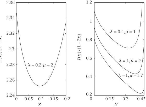
Figure_6.1. _{Behaviour ofI(x)/(r−x(r−r0))againstxforr0= −1,}

r=1, and varying values ofλandµ.

Table_6.1._{Value ofxat whichI(x)/(1−2x)attains the minimum}

and the corresponding minimum for different values ofλandµ.

λ µ x I(x)/(1−2x)

1.0 1.7 0.44469 0.22213441870537 0.4 1.0 0.32968 0.70963293158894 1.0 2.0 0.39347 0.43275212957147 0.8 2.0 0.32968 0.70963293158894 0.2 2.0 0.09516 2.25216846109190

when r =1= −r0, withλ=1 and µ =1.7, we findx =0.44469, quotient = 0.22213441870537, that is,P (fluid> t)≈exp(−0.22213441870537t). Ob-serve that for sufficiently small values oft, exp(−0.22213441870537t)turns out to be a straight line.

Figure 6.1depicts the behaviour of this functionI(x)/(r−x(r−r0))against

x forr =1= −r0and the varying values ofλ andµ whereI(x)is given by (6.5).Table 6.1gives the value ofxat which the quotient attains minimum for the various parameter values.

The governing system of differential-difference equations given by (3.5) can be written in the matrix notation as

dF(x) dx =R

−1_QT_{F(x), (7.1)}

whereF(x)=[F0(x), F1(x), F2(x), . . .]T_{,R=diag{r0, r , r , . . .}, andQ denotes}

the infinitesimal generator of the background birth and death process given by

Q=       

−λ0 λ0

µ1 −λ1+µ1 λ1

µ2 −λ2+µ2 λ2

. ._. . ._. . ._.      

. (7.2)

The capacity of the background birth and death process is unrestricted in our theoretical study. However, for the purpose of numerical investigations, we truncate the size of the process by a finite quantity, sayN. HenceR−1_QT_takes

the form

R−1QT=                

−λ0

r0

µ1 r0 λ0

r −

λ1+µ1 r

µ2 r

. ._. . ._. . ._.

µN r λN₋1

r −

µN r

               

N+1

. (7.3)

Mitra [10] have shown that R−1_QT _{has exactly N}

+ negative eigenvalues, N₋−1 positive eigenvalues, and one zero eigenvalue, whereN₊ is the cardi-nality of the setS+≡ {j∈᏿:rj>0}andN−is that ofS−≡ {j∈᏿:rj<0}.

Suppose thatξj,j=0,1,2, . . . , N, are the eigenvalues of the matrixR−1_QT

such that

ξj<0, j=0,1, . . . , N−1, ξN=0 (7.4)

andy_=[y

0, y1, . . . , yN]T,z =[z0, z1, . . . , zN]are the right and the left

eigen-vectors of the matricesR−1_QT _andQT_R−1_{, respectively, corresponding to the}

eigenvalueξ.

Then,

y

0=1=z0 for∈᏿,

y_j=Bj

ξ

cj0 , z j=

r0Bjξ

r cj0 forj, ∈᏿\{0},

where the polynomialsBj(s)are recursively defined as follows:

B0(s)=1,

B1(s)=

s+λ0

r0 B0(s),

B2(s)=

s+λ1+_rµ1 B1(s)−λ0µ1_r0r B0(s),

Bj(s)=

s+λj−1+µj−1

r Bj−1(s)−

λj−2µj−1

r2 Bj−2(s), j=3,4, . . . , N,

BN₊1(s)=

s+µN

r BN(s)− λN₋1µN

r2 BN−1(s)

(7.6)

and

cj0=µ1µ2···µj

r0rj−1 . (7.7)

From the knowledge of the eigenvalues, left and right eigenvectors, the equi-librium distribution of the buffer occupancy is given by (see [8])

Fj(x)=pj+

N−1

=0

β_jexpξx forj∈᏿, x≥0, (7.8)

where

β j=yj

r0F0(0) rN_k=0y

kzk

. (7.9)

The unknownF0(0)representing the distribution of the buffer occupancy when the buffer is empty and the background process is in state zero is obtained as

F0(0)=p0

π0r0+rNj=1πj

r0 . (7.10)

Determination of eigenvalues. _{We determine the eigenvalues ofR}−1_QT from its associated characteristic polynomial denoted byP(s):

P(s)=

s+λ0_r0 −µ1_r0

−λ0_r s+λ1+_rµ1 −µ2_r . ._. . ._. . ._.

−µN

r

−λN−1 r s+

µN r

_N+1

It can be written as

P(s)=

s+λ0_r0 λ0_r0

µ1 r s+

λ1+µ1 r

λ1 r

. ._. . ._. . ._.

λN₋1 r µN

r s+ µN r _N+1

. (7.12)

Doing the operations: (1) rowi=(rowi)+(rowi+1)fori=1,2, . . . , N, (2) diminishing the second column by the first, the third column by the new second column, and so on in the above determinant, we get

P(s)=s×

s+λ0_r0+µ1_r µ1_r

λ1

r s+

λ1 r + µ2 r µ2 r . ._. . ._. . ._.

µN₋1 r λN−1

r s+ λN−1

r + µN r N . (7.13)

Thus zero is an eigenvalue ofR−1_QT_{. The above determinant is sign-symmetric}

and hence can be written as

P(s)=s×

s+λ0

r0+ µ1 r λ1µ1 r λ1µ1

r s+

λ1 r + µ2 r λ2µ2 r . ._. . ._. . ._.

λN₋1µN₋1 r

λN−1µN−1

r s+

λN−1 r + µN r N . (7.14)

The other eigenvalues ofR−1_QT_{are determined from the associated real}

sym-metric matrix of this reduced determinantP(s)by using the method of bisec-tion suggested by Evans et al. [4] with suitable modificabisec-tions.

Determination of eigenvectors. LetM(s)=((aij))denote the matrix

of the eigenvector of the underlying matrices, the polynomialsBj(s)play a major role. Since the system of equations given by (7.6) is an underdetermined system, at least one of the equations is redundant. If thekth equation is redun-dant, we may assumeBk(s)=1 and solve the rest of the equations. Fernando [5] provides a method to overcome the instability that arises because of this particular normalization. This is achieved by computing the diagonal entries of the matrixᏲ, which is obtained by elementwise reciprocation of the inverse ofM(s)T_{based onLDUandU DLfactorization of the tridiagonal matrixM(s).}

We consider theLDUfactorization ofM(s). The diagonal elementsdi(s)of

Dare given recursively as

d0(s)=a0,0,

di(s)=ai,i−ai−1,iai,i−1

di−1(s) , fori=1,2, . . . , N,

(7.15)

where s is the eigenvalue of the matrix R−1_QT_{. Now, we consider theUDL}

factorization ofM(s). The diagonal elementsδi(s)are given recursively as

δN(s)=aN,N,

δi(s)=ai,i−ai+1,iai,i+1

δi+1(s) , fori=N−1, N−2, . . . ,0.

(7.16)

Then the diagonal elementsηi(s)of the matrixᏲare given by

η1(s)=δ1(s),

ηi(s)=δi−ai−1,iai,i−1

di−1(s) , fori=2,3, . . . , N+1.

(7.17)

The following algorithm may be used for computingBj(s)with suitable nor-malization suggested by the algorithm.

Algorithm_7.1. _{(1) Computeηk}=_min0≤i≤N{_ηi}_.

(2) SetBk(s)=1, wherekis corresponding to the suffixkofηkin step (1). (3) Compute otherBj(s)using

Bj(s)= −aj,j_dj(s)+1Bj+1(s), j=k−1, k−2, . . . ,0,

Bj(s)= −aj,j_δj(s)−1Bj−1(s), j=k+1, k+2, . . . , N.

(7.18)

To visualize the foregoing discussion, we plot the graphs of buffer content distribution for the two models by assuming certain values for the parameter

0 10 20 30 40 50 60 70 80 Buffer contentx

10−14 10−12 10−10 10−8 10−6 10−4 10−2 100

log

10

P(

C

>

x

)

λ =

0 .₂

,µ =

2 λ

= 0

.₂ ,µ

= 2

λ₌

0_. 8_,µ

= 2

λ₌

0_. 8_,µ

= 2

λ₌

1_,µ =₂

λ₌

1_,µ =₂

λ₌

0_.4 ,µ

=₁

λ₌

0_.4

,µ₌

1 λ₌

1_{, µ=}

1.7

λ₌₁ , µ₌

1.7

Model 1λn=λ;µn=nµ Model 2λn=λ/n+1;µn=µ

Figure_7.1._{Buffer content distribution withr0= −1,r=1, andN=30.}

Appendices

A. We verify below that ˆF0(s)and ˆF1(s)satisfy (4.2). Consider

r0s+λF0(s)ˆ −r0F0(0)=µF1(s).ˆ (A.1)

Substituting for ˆF0(s)and ˆF1(s)from (4.8), we need to verify

r0s+λ1F1

2; λr s

(r s+µ)2+2;− λµ (r s+µ)2

− λµ

(r s+µ)

21F13;λr s/(r s+µ)2_{+3;−λµ/(r s+µ)}2 λr s/(r s+µ)2₊₂

=s

r

_{λr s}

(r s+µ)2+1 +

r0−r1F1

2; λr s

(r s+µ)2+2;− λµ (r s+µ)2 .

(A.2)

Leta=2,c=λr s/(r s+µ)2_{+2, andz= −λµ/(r s+µ)}2_{. Then we need to verify}

r0s+λ1F1(a;c;z)− λµ

(r s+µ)

a1F1(a+1;c+1;z) c

=sr (c−1)+r0−r1F1(a;c;z).

Observe that

r0s+λ1F1(a;c;z)− λµ

(r s+µ)

a1F1(a+1;c+1;z) c

=_{c(r s}1_+µ)cr0s+λ(r s+µ)1F1(a;c;z)−aλµ1F1(a+1;c+1;z)

= 1

c(r s+µ)

cr0s(r s+µ)1F1(a;c;z)+cλr s1F1(a;c;z)

+λµc1F1(a;c;z)−a1F1(a+1;c+1;z).

(A.4)

Using identity (2.5), we obtain

r0s+λ1F1(a;c;z)−_{(r s}λµ_+µ)a1F1(a+_c1;c+1;z)

= 1

c(r s+µ)

cr0s(r s+µ)1F1(a;c;z)+cλr s1F1(a;c;z)

+λµ(c−a)1F1(a;c+1;z)

= 1

c(r s+µ)

cr0s(r s+µ)1F1(a;c;z)

+cλr s1F1(a;c;z)−λr sz1F1(a;c+1;z)

=_{c(r s}1_+µ)cr0s(r s+µ)1F1(a;c;z)

+λr sc1F1(a;c;z)−z1F1(a;c+1;z).

(A.5)

Using (2.6), we get

r0s+λ1F1(a;c;z)−_{(r s}λµ_+µ)a1F1(a+_c1;c+1;z)

= 1

c(r s+µ)

cr0s(r s+µ)1F1(a;c;z)+cλr s1F1(a−1;c;z)

=s

r0 1F1(a;c;z)+_{r s}λr_+µ1F1(a−1;c;z)

.

(A.6)

Adding and subtractingr1F1(a;c;z)yields

r0s+λ1F1(a;c;z)− λµ

(r s+µ)

a1F1(a+1;c+1;z) c

=sr0−r1F1(a;c;z)+r

1F1(a;c;z)+ λ

(r s+µ)1F1(a−1;c;z)

.

Using (2.7), we obtain

r0s+λ1F1(a;c;z)− λµ (r s+µ)

a1F1(a+1;c+1;z) c

=sr0−r1F1(a;c;z)+r (c−a+1)

=sr0−r1F1(a;c;z)+r (c−1).

(A.8)

Hence the verification.

B. We verify below that ˆG0(s)and ˆG1(s)satisfy (5.2). Consider

r0s+λG0(s)ˆ −µG1(s)ˆ =r0G0(0). (B.1)

Substituting for ˆG0(s)and ˆG1(s)from (5.8), we need to verify

r0s+λ1F1

1;r s

µ +1;− λ µ −

λ r s/µ+11F1

2;r s

µ +2;− λ µ

=s

r+r0−r1F1

1;r s

µ +1;− λ µ .

(B.2)

Observe that

r0s+λ1F1

1;r s

µ +1;− λ µ −

λ r s/µ+11F1

2;r s

µ +2;− λ µ

=_{r s/µ}1₊₁r0s+λr s

µ +1 1F1

1;r s

µ +1;− λ

µ −λ1F1

2;r s

µ +2;− λ µ

= 1

r s/µ+1

r0s

_{r s}

µ +1 1F1

1;r s

µ +1;− λ µ

+λ

_{r s}

µ +1 1F1

1;r s

µ +1;− λ µ −1F1

2;r s

µ +2;− λ

µ .

(B.3)

Using identity (2.5) witha=1,c=r s/µ+1, andz= −λ/µ, we obtain

r0s+λ1F1

1;r s

µ +1;− λ µ −

λ r s/µ+11F1

2;r s

µ +2;− λ µ

= 1

r s/µ+1

r0s

_{r s}

µ +1 1F1

1;r s

µ +1;− λ µ +λ

r s µ 1F1

1;r s

µ +2;− λ µ .

Adding and subtracting the termr (r s/µ+1)1F1(1;r s/µ+1;−λ/µ)and using identity (2.6), we obtain

r0s+λ1F1

1;r s

µ +1;− λ µ −

λ r s/µ+11F1

2;r s

µ +2;− λ µ

= s

r s/µ+1

r0−rr s

µ +1 1F1

1;r s

µ +1;− λ µ +r

_{r s}

µ +1

=s

r+r0−r1F1

1;r s

µ +1;− λ µ .

(B.5)

Hence the verification.

Acknowledgments We thank the referees for their constructive criticism.

The comments of one of the referees are gratefully acknowledged, which led to the discussion on the asymptotic analysis of our model. P. R. Parthasarathy thanks the Department of Science and Technology, Indian Institute of Tech-nology, India, for the financial assistance during the preparation of this paper.

References

[1] M. Abramowitz and I. A. Stegun (eds.),Handbook of Mathematical Functions, with Formulas, Graphs, and Mathematical Tables, National Bureau of Standards Applied Mathematics Series, vol. 55, Superintendent of Documents, U.S. Government Printing Office, District of Columbia, 1965.

[2] L. C. Andrews,Special Functions of Mathematics for Engineers, 2nd ed., McGraw-Hill, New York, 1992.

[3] E. A. van Doorn and W. R. W. Scheinhardt,A fluid queue driven by an infinite-state birth-death process, Teletraffic Contributions for the Information Age (Proc. 15th International Teletraffic Congress, Washington, DC) (V. Ra-maswami and P. E. Writh, eds.), Elsevier, Amsterdam, 1997, pp. 465–475. [4] D. J. Evans, J. Shanehchi, and C. C. Rick,A modified bisection algorithm for the

determination of the eigenvalues of a symmetric tridiagonal matrix, Numer. Math.38(1981/1982), no. 3, 417–419.

[5] K. V. Fernando,On computing an eigenvector of a tridiagonal matrix. I. Basic results, SIAM J. Matrix Anal. Appl.18(1997), no. 4, 1013–1034.

[6] F. Guillemin and D. Pinchon,Continued fraction analysis of the duration of an excursion in anM/M/∞system, J. Appl. Probab. 35(1998), no. 1, 165– 183.

[7] C. H. Lam and T. T. Lee,Fluid flow models with state-dependent service rate, Comm. Statist. Stochastic Models13(1997), no. 3, 547–576.

[8] R. B. Lenin and P. R. Parthasarathy, A computational approach for fluid queues driven by truncated birth-death processes, Methodol. Comput. Appl. Probab.2(2000), no. 4, 373–392.

[9] ,Fluid queues driven by anM/M/1/Nqueue, Mathematical Problems in Engineering6(2000), 439–460.

[10] D. Mitra,Stochastic theory of a fluid model of producers and consumers coupled by a buffer, Adv. in Appl. Probab.20(1988), no. 3, 646–676.

[12] S. Resnick and G. Samorodnitsky,Steady-state distribution of the buffer content forM/G/∞input fluid queues, Bernoulli7(2001), no. 2, 191–210. [13] B. Sericola and B. Tuffin,A fluid queue driven by a Markovian queue, Queueing

Systems Theory Appl.31(1999), no. 3-4, 253–264.

[14] A. Shwartz and A. Weiss,Large Deviations for Performance Analysis, Stochastic Modeling Series, Chapman & Hall, London, 1995.

P. R. Parthasarathy: Department of Mathematics, Indian Institute of Technology, Madras, Chennai 600 036, India

E-mail address:[email protected]

K. V. Vijayashree: Department of Mathematics, Indian Institute of Technology, Madras, Chennai 600 036, India