EXPLICIT GEODESIC FLOW-INVARIANT DISTRIBUTIONS
USING
SL
2(
R
)
-REPRESENTATION LADDERS
ALVARO ALVAREZ-PARRILLA
Received 6 August 2003 and in revised form 10 March 2005
An explicit construction of a geodesic flow-invariant distribution lying in the discrete series of weight 2kisotopic component is found, using techniques from representation theory of SL2(R). It is found that the distribution represents an AC measure on the unit tangent bundle of the hyperbolic plane minus an explicit singular set. Finally, via an av-eraging argument, a geodesic flow-invariant distribution on a closed hyperbolic surface is obtained.
1. Introduction
Flow-invariant quantities play a major role in dynamics, namely, in answering ergodic questions, and are related, via thecohomological equation, to the problem of describing time changes for flows (see, e.g., [3,4,5,10] and the references therein).
On the other hand, the study of geometrically invariant objects arising from automor-phic forms has been a major player in some questions arising in Riemann surfaces and in physics [1,6,7,8,9,13,15,17,22,20,21,25].
In particular, it is well known that geodesic flow-invariant quantities appear quite nat-urally in quantum chaos: geodesic flow is a model for the time evolution of a classical mechanical system; while the time evolution of the quantum mechanical system is given in terms of the eigenfunctions of a certain selfadjoint operator. The transition between a classical mechanical system and the quantum version of the same system involves a method commonly known as quantization. The inverse process, that of going from a quantum mechanical system to a classical system, involves a limit which the physicists would like to claim as unique. (This is known as thecorrespondence principleor the semi-classical limit.) A central problem in physics since the late twenties has been trying to understand this transition. One of the main stumbling blocks seems to stem from the fact that there are many possible quantizations for the same classical system and it is not clear which of these should be the “correct one,” furthermore the question of the uniqueness of the limit is also relevant. A mathematical approach to the problem can be stated as theunique quantum ergodicityquestion, where one is interested in finding the weak* limit points of microlocal lifts of eigenfunctions of the hyperbolic Laplacian
Copyright©2005 Hindawi Publishing Corporation
[2,8,13,16,18,23,24,25]. It is well known that such limits must be geodesic flow-invariant measures on the unit (co-)tangent bundle of the Riemann surface [19], how-ever, it is unknown which invariant measures actually occur.
On this matter, Zelditch, ˇSnirel’man, and Colin de Verdi`ere [2,18,23] independently showed that almost all limits are Liouville measures for a compact hyperbolic surface. There is evidence supporting that this limit is unique for M=PSL2(Z)\PSL2(R) (see [13,16]), while on the other hand, Jakobson [8] showed that for the flat tori, the possible limits are of the formν=φ(x)dVol, whereφ(x) is a trigonometric polynomial satisfying a rigid geometric condition.
As a further step in trying to understand the possible measures that could arise from such a limit, we undertake the study of geodesic flow-invariant distributions lying com-pletely in the discrete series of weight 2kisotopic component of SL2(R) by explicitly con-structing them and examining some of their properties. This is done using a “ladder” construction on the (square root of the) unit tangent bundle of the hyperbolic plane, by methods based on the representation theory of SL2(R).
The background material is presented inSection 2, while the actual construction is carried out inSection 3 and can be summarized as follows: essentially, a distribution onT1∗Hthat lies completely in the discrete series unitary representation is constructed, then it is made geodesic flow-invariant by requiring it to be in the kernel of the operator corresponding to geodesic flow. The first requirement is met by using a “ladder” con-struction in which a suitable holomorphic form of a given weight 2kis raised to weights 2k+n,na positive integer, and these are all summed with a yet unspecified coefficient to form an infinite series. The requirement that this series be geodesic flow-invariant char-acterizes completely the coefficients (up to a constant) and further analysis shows that this is in fact a distribution of order 0 with singularities of logarithmic type or milder (Theorem 3.8). Furthermore, the singular set has a simple geometrical description (Fig-ures2.1and2.2). Finally, a geodesic flow-invariant distribution is obtained on a closed hyperbolic surface by the usual procedure of averaging over the group, this result is pre-sented asTheorem 3.12.
2. Background
As mentioned in the introduction, we will be using the representation theory of SL2(R), hence we introduce some terminology that may not be common to all readers.
2.1. Notation and terminology. Let G=SL2(R)= {a b c d
|ad−bc=1, a,b,c,d∈R}, and let K=SO(2)= {−cossinθθsincosθθ
|θ∈[0, 2π)} ∼=S1⊂C be the orthogonal group. No-tice thatKis the stabilizer ofi∈H, whereH= {z∈C|Imz >0}is the upper half-plane. The action ofGonHis by fractional linear transformations. We adopt the usual con-vention thatz=x+iy, so the action ofa bc d∈Gis given bya bc d:z→(az+b)/(cz+d). Notice that this action factors through the center, hence it is an action of PSL2(R)=
SL2(R)/±Id.
Letµg(z)=cz+d; it is called theautomorphy factorand satisfies the cocycle relation
ψ
Θ
[image:3.468.132.334.72.184.2]Singular set on upper half-plane
Figure 2.1. Singular setk,γ0fort1,γ0onT ∗
1H. Dotted vectors representθ−ψ=j(π/2).
0 π/2 π
ψ
0
π/2
π
3π/2 2π
Θ
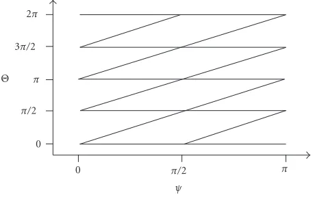
Figure 2.2. Singular setk,γ0fortk,γ0,k=1, 2, in the (ψ,θ) coordinates of
T1∗H.
SinceK fixesi∈H, then there is a natural identification between SL2(R)/K andH given bygK→gi=(ai+b)/(ci+d). In fact we can identify SL2(R) withT1∗Hthe square root (the double cover) of the unit cotangent bundle via the mapg→(gi, (µg(i)/µg(−i))α) forα∈S1⊂C. Note thatµ
g(i)/µg(−i)=(dg/dz)1/2(dg/dz¯)−1/2=(dz/dz¯ )1/2. This can also be seen by recalling [12] that an elementg∈SL2(R) has the unique Iwasawa decomposi-tion
g=
a b
c d
=
1 x
0 1
y1/2 0 0 y1/2
cosθ sinθ
−sinθ cosθ
, (2.1)
hence the rule
x+iy=y1/2eiθ(a+ib), y−1/2eiθ=d−ic, (2.2)
[image:3.468.120.350.238.382.2]Next, we define anautomorphic formon SL2(R)for the groupΓwithweightl∈Cas a function fl: SL2(R)→Csatisfying
(i) (leftΓ-invariance)fl(γg)=fl(g) for allγ∈Γandg∈G;
(ii) (right action by K) fl(gk)=µk(i)−lfl(g) for all k∈K. Notice thatµk(i)=eiθ sincek=cosθ sinθ
−sinθcosθ
;
(iii) flsatisfies an SL2(R)-invariant differential equation.
With this definition in mind, it is easy to recover the more common definitions of an automorphic form as a function onH. The key lies in the following procedure that takes functions defined onHand lifts them to functions on SL2(R) and vice versa:
functions onH−→ weightlfunctions on SL2(R),
f(z)−→ fl(g) := f(gi)µg(i)−leilθ,
(2.3)
where z=gi for some g ∈G. It is interesting to note that we can rewrite fl(g)=
f(z)yl/2eilθ, and that f
ltransforms on the right according to the character
cosθ sinθ −sinθcosθ
→
eikθofK. With the procedure described above, we have then that anautomorphic formon Hfor the groupΓwithweightl∈Cis a function f :H→Csatisfying
(i) f(γz)=µγ(z)lf(z) for allγ∈Γ;
(ii) f is the solution to an SL2(R)-invariant differential equation.
Note that further regularity and growth properties follow from the last condition in each of the two definitions.
As stated, this definition of automorphic form is very wide; by allowing for different growth conditions, we can change the number of automorphic forms that are allowed; the more strict the condition, the less forms satisfying it.
2.2. Some representation theory ofSL2(R). LetM=Γ\H, whereΓis a cofinite group of isometries ofH. Then the Lie Algebra ofMis locally identified withp, the space of sym-metric matrices with trace zero, contained insl2(R), which in turn enables us to use the techniques of representation theory. In accordance with Bargmann’s classification theo-rem (see, e.g., [12, Theorem IV.6.8]), there are four different types of unitary representa-tions of SL2(R): discrete series, mock discrete series, principal series, and complementary series. All of these are infinitesimally isomorphic to some explicit subspaces of functions on SL2(R). The explicitness of these subspaces is what will enable us to work with them [11,12].
Consider the Iwasawa decomposition of SL2(R)=ANK, hence ifg∈SL2(R), then
g=uy x0 1r(θ), wherer(θ)=cosθ sinθ −sinθcosθ
∈Kand abusing notationu=u0 0u
∈A, note that y,u >0. Lets∈C. DefineH(s) to be the space of functions f on SL2(R) such that
f|K∈L2(K), and satisfying the condition f(g)= f(u0 1y x
r(θ))=ys+1/2f(r(θ)). In par-ticular, letψn∈H(s) be the function such thatψn(r(θ))=einθ. Letπsbe the representa-tion of SL2(R) onH(s) by right translation. By Bargmann’s classification theorem, the dis-crete series representation of weightmcorresponds to±s=m−1, wheremis an integer greater than or equal to 2. Consider the following two subspaces ofH(m−1):
H(m)= n≥m n≡mmod 2
ψn
, H(−m)=
n≤−m n≡mmod 2
ψn
The subspaceH2k≡H(2k)⊕H(−2k)⊆H(2k−1) is calledthe discrete series unitary
repre-sentation of weight2k. Notice that if f ∈H(2k), then ¯f ∈H(−2k). Recall that this is just a
realizationof the discrete series unitary representation.
3. The construction
LetV be the space of functions on SL2(R) such that f|K∈L2(K) and that are also ge-odesic flow-invariant. Then SL2(R) acts onV by right translation. Ifπis an irreducible representation of SL2(R) onV, thenV(π)=Image(ϕ), withϕ∈Hom(π,V), is the
π-isotopic component ofVand consists of “copies” of theπirreducible subspaces. Denote byH(2k−1)(π2k) thediscrete series of weight2kisotopic component inV, and byH(2k−1)(π2k) the corresponding distributions. Consider the formal sumT= nfn, with fn∈H(2k−1)(π2k) for alln. By abusing notation, we defineTas a distribution on SL2(R) associated to the formal sum. We will say thatthe distributionTlies completely in
H(2k−1)(π2k) if the partial sumTN= n≤N fn∈H(2k−1)(π2k) for allN >0. It is now possible to specifically state the problem addressed in this paper.
Main question. Suppose we have a geodesic flow-invariant distribution lying completely in the discrete series of weight 2kisotopic componentH(2k−1)(π2k). What can we say about the distribution?
3.1. The plan of action. In order to answer the above question, an explicit construction of a geodesic flow-invariant distribution is carried out. The idea behind the construction is as follows: start with a suitable holomorphic form on a hyperbolic manifoldM and then via a “ladder” construction obtain the distribution lying in the discrete series of weight 2k. SinceM is a hyperbolic quotient, work onHby requiring the objects to be automorphic forms of weight 2k.
The use of relative Poincar´e series allows the construction of such automorphic forms; recall that the Petersson series,Θk,γn, are automorphic forms of weight 2kassociated to
primitive hyperbolic elementsγn∈Γ(for further details, see [9]).Θk,γn is constructed by
summing over the group the functionQ−kγn(z)=(cz2+ (d−a)z−b)−k, associated to the hyperbolic elementγn=
a b c d
. By conjugating the group with an appropriate element, it is possible to use a primitive hyperbolic elementγ0∈Γwhose axis is the imaginary axis (in the upper half-plane model of H). In this case,Qγ0(z)=(a−1−a)z. Thus the construction is carried out usingΘk,γ0.
Since the representation theory of SL2(R) is to be used, we use the lifting procedure, outlined in (2.3), to lift forms onHto functions on SL2(R), as well as the identifica-tion of SL2(R) withT1∗Hthe square root (double cover) of the unit cotangent bundle ofH. This allows us to establish a correspondence between tensors onHand functions on SL2(R): let f(z)dzkbe a symmetrick-tensor onH, consider first thebalancedtensor
f(z)ykdzk/2dz¯−k/2 (recall that the hyperbolic metric isds=y−1dz1/2dz¯−1/2). Then asso-ciate, under the identification of SL2(R) withT1∗H, the weight 2k function on SL2(R) given byΨk(z,θ)=f(z)ykei2kθ. The functionΨk(z,θ) on SL2(R) is called thelift of f.
Under this procedure, the functionQ−kγ0(z) is lifted (up to a constant) to the function
of the Petersson seriesΘk,γ0, and use the techniques of representation theory of SL2(R) to make the “ladder” geodesic flow-invariant.
Instead of summing over the group immediately (and obtaining the lift ofΘk,γ0(z)), we opt to first obtain its “ladder” inH2k.
In order to construct the “ladder”, we will need to compute the action of the following elements of the Lie algebra of SL2(R):E+=1i −i1
,E−=−i1 −−i1
, andW=0 1 −1 0
. The infinitesimal representationdπs acts on elements of H(s) via the Lie derivative, hence abusing notation and denoting byE+,E−, andWthe Lie derivatives ofE+,E−, andW, respectively, we have
E+=ei2θ
2(z−z¯)∂
∂z+
1
i ∂ ∂θ
,
E−=e−i2θ
−2(z−z¯)∂
∂z¯− 1
i ∂ ∂θ
,
W= ∂
∂θ,
(3.1)
these are the “raising,” “lowering,” and “weight” operators, respectively, (since they raise, lower, and pick out the weights of theψn). Notice that one can think of the operatorE+ as generalizing the complex exterior differential∂which maps forms of typedzkto forms of typedzk+1, also note that formally we haveE
−=E+, and since we are interested in calculating ladders inH2k=H(2k)⊕H(−2k), then it follows by the above remark and the following standard lemma (whose proof can be found in, say [11,12]), that it is only necessary to calculate inH(2k).
Lemma3.1 (discrete series ladder). Letu∈H(s). Suppose that
(1)Wu=i2k u, forkinteger,k≥1,
(2)E−u=0. Then,V= En
+u ⊕ En−u,n=0, 1, 2,. . ., is a representation ofsl2(R)isomorphic toH2k=
H(2k)⊕H(−2k).
With this in mind, the construction should proceed as follows.
(1) We will start with theγ0-invariant functiongk,γ0, and proceed to construct its ladder
tk,γ0(z,θ)=
m≥0
amEm+gk,γ0(z,θ). (3.2)
(2) Next we will determine the coefficientsam which make the ladder geodesic flow-invariant (Section 3.3).
(3) Finally sum over the group to obtain the geodesic flow-invariant distribution on
Mlying only inH2k(Section 3.4).
Letk∈Z+be fixed. Consider the polynomials
qn(x)= n
j=0
n−j+k−1
k−1
j+k−1
k−1
xj. (3.3)
Lemma3.2. The polynomials defined by (3.3) satisfy the following recursion relation:
q0(x)=1,
(n+ 1)qn+1(x)=(n+k+kx)qn(x)−x(1−x)dxd qn(x).
(3.4)
Proof. The proof is a simple induction argument onn.
Lemma 3.3 (generating function for polynomials). The polynomials defined by (3.3)
have generating function
(1−xy)−k(1−y)−k=
n≥0
qn(x)yn. (3.5)
Proof. Expand (1−y)−k and (1−xy)−kin a power series about the origin, and obtain the product. Notice that the radius of convergence of each series is 1, hence the series
converges for|y|<1, and|x|<1/|y|.
Now consider the polynomials
pn(x)=(1−x)2k−1qn(x). (3.6)
We have the following lemma.
Lemma3.4. The polynomialspn(x)=(1−x)2k−1qn(x)satisfy (i) pn(x)is a polynomial inxof degreen+ 2k−1, (ii) pn(x)has exactly2kterms, that is,
pn(x)=bn,0+bn,1x+···+bn,k−1xk−1+bn,n+kxn+k
+bn,n+k+1xn+k+1+···+bn,n+2k−1xn+2k−1,
(3.7)
(iii)the coefficientsbn,j, for j=1, 2,. . .,k−1,n+k,n+k+ 1,. . .,n+ 2k−1, are
polyno-mials innof degree≤k−1.
Proof. From (3.6), and since deg(pn)=2k−1 + deg(qn), (i) follows because deg(qn)=n. In the proof of statement (ii), we will drop the index corresponding tonin the coeffi -cients of the polynomialpn(x), that is, we will writebjinstead ofbn,j(sincenis fixed).
In order to prove this statement, we first need a recursion relation for the polynomials
pn, we obtain this from (3.4). From the definition ofpn(x), we have that
qn(x)=(1−x)−(2k−1)pn(x),
d
dxqn(x)=(1−x)
−(2k−1) d
dxpn(x) + (2k−1)(1−x)
−2kp n(x),
so substituting in (3.4), we obtain the desired recursion relation for the polynomialspn:
p0(x)=(1−x)2k−1,
(n+ 1)pn+1(x)=
n+k+ (1−k)xpn(x)−x(1−x)dxd pn(x).
(3.9)
We now proceed by induction onn. Forn=0, the result follows by the binomial theorem as follows:
p0(x)=(1−x)2k−1=
2k−1
j=0 (−1)j
2k−1
j
xj. (3.10)
Next we considern=m+ 1. By induction hypothesis,
pm(x)=b0+b1x+···+bk−1xk−1+bm+kxm+k
+bm+k+1xm+k+1+···+bm+2k−1xm+2k−1
(3.11)
hence substituting in (3.9) and collecting terms of the same degree,
(m+ 1)pm+1(x)=(m+k)b0+
(m+k−1)b1−(k−1)b0
x
+(m+k−2)b2−(k−2)b1
x2+···
+(m+ 1)bk−1−bk−2
xk−1+(m+ 1)b
m+k−bm+k+1
xm+k+1
+(m+ 2)bm+k+1−2bm+k+2
xm+k+2+···
+(m+k−1)bm+2k−2−(k−1)bm+2k−1
xm+2k−1
+ (m+k)bm+2k−1xm+2k.
(3.12)
So, indeedpn(x) has exactly 2kterms.
Finally to prove statement (iii), we know thatpn(x)=(1−x)2k−1qn(x), hence by (3.3) and by the binomial theorem, we have
pn(x)= 2k−1
i=0 (−1)i
2k−1
i xi n j=0
n−j+k−1
k−1
j+k−1
k−1
xj
=
n+2k−1
m=0
i+j=m (−1)i
2k−1
i
n−j+k−1
k−1
j+k−1
k−1
xm,
(3.13)
so in fact
bn,m=
i+j=m (−1)i
2k−1
i
n−j+k−1
k−1
j+k−1
k−1
and since
n−j+k−1
k−1
=(n−j+ 1)(n−j+ 2)(n−j+ 3)···(n−j+k−1)
(k−1)-terms
, (3.15)
then indeedbn,mis a polynomial innof degree≤k−1.
3.3. Explicit construction onSL2(R). Letγ0∈Γbe a hyperbolic element whose axis is the imaginary axis onH. Consider the function on SL2(R)
gk,γ0(z,θ)=
ykei2θk
zk , (3.16)
(recall that this is the lift ofQ−kγ0(z)), and its ladder
tk,γ0(z,θ)=
m≥0
amEm+gk,γ0(z,θ). (3.17)
Notice that, as required byLemma 3.1,Wgk,γ0=i2k gk,γ0andE−gk,γ0=0.
To find the coefficients am, we will make use of the fact that we requiretk,γ0 to be geodesic flow-invariant. The operator generating geodesic flow is given in terms ofE+ andE−byG=(E++E−)/2. Hence we require thatGtk,γ0=0, or equivalently,
n≥0
E++E−anE+ngk,γ0=0. (3.18)
This will enable us to determine explicitly the coefficients that make the ladder (3.17) geodesic flow-invariant.
Remark 3.5. It is to be noted that since (E++ E−)/2=1 00−1
, then the requirement that the ladder (3.17) is to be geodesic flow-invariant can be stated as saying that it must be
A-invariant (whereA <SL2(R) is the subgroup of diagonal matrices).
Lemma3.6 (geodesic flow-invariant coefficients). The coefficients that make the ladder
(3.17) geodesic flow-invariant are given by
an=
(k−1/2)!
24m(m+k−1/2)!m! ifn=2m,
0 ifn=2m+ 1,
(3.19)
form∈Z. In other words, with the above choice of coefficients (formal)A-invariance of the ladder (3.17) exists (up to the choice ofa0, see proof).
Proof. The proof of the lemma proceeds as follows.
SinceE+andE−are the raising and lowering operators, they satisfy the commutation relation
whereW=∂/∂θ corresponds to the element−0 11 0
and “picks out the weight” of the function on which it acts (soWgk,γ0=i2k gk,γ0).
Thus from (3.18), we obtain the following recursion relation:
a0E−gk,γ0=0,
a1E−E+gk,γ0=0,
anEn++1gk,γ0+an+2E−
En++2
gk,γ0=0, ∀n≥0.
(3.21)
From this and the fact thatE−gk,γ0=0, sincegk,γ0is a holomorphic form, we have that
a0is a free coefficient. Without loss of generality, we leta0=1. By repeated use of (3.20), we have
E−En++2
gk,γ0=E−E+
En+1 +
gk,γ0=
E+E−+ 4iWEn++1gk,γ0
=E2
+E−En++ 4iE+WEn++ 4iWEn++1
gk,γ0 ..
.
=
En++2E−+ 4i n+1
j=0
E+jWEn−j+
gk,γ0,
(3.22)
with the convention thatE0
+≡1. But sincegk,γ0is a holomorphic form, thenE−gk,γ0=0, and sinceW“picks out” the weight,WEm
+gk,γ0=2i(k+m)gk,γ0, then
E−En++2
gk,γ0=4i n+1
j=0
2i(k+j)En+1 + gk,γ0
= −22(n+ 2)2+ (2k−1)(n+ 2)En++1gk,γ0.
(3.23)
Hence substituting in (3.21), we obtain
an−22(n+ 2)2+ (2k−1)(n+ 2)an+2En++1gk,γ0=0 ∀n≥0, (3.24)
that is,
an= an−2
22[n2+ (2k−1)n] ∀n≥2. (3.25)
Sincea0=1, we obtain that forn=2m,
an= n/2
j=1
22(2j)2+ 2j(2k−1)−1= (k−1/2)!
On the other hand fornodd, we have from (3.21) thata1E−E+gk,γ0=0, and by the same arguments as above, we see that
0=a1E−E+gk,γ0=a1
E+E−+ 4iWgk,γ0=4ia1Wgk,γ0 (3.27)
hencea1=0, and by (3.25),an=0 fornodd.
This proves the lemma.
Remark 3.7. Notice that in the proof of the above lemma, we have used the facts that
gk,γ0 is an eigenvector of the Casimir operatorωand thatωcommutes withE+,E−, and W. Furthermore, the determination of the coefficients (and hence of the ladder (3.17)) is unique up to the choice of the coefficienta0.
It will now be convenient to introduce the change of variables α=z/z¯ =e−i2ψ and
β=ei2θ, wherez=x+iy=reiψ, andθis the fiber variable forT∗
1H. Recall that since
y >0, then 0< ψ < π, andθrepresents the “direction” in the unit cotangent bundle, so 0≤θ < π(seeFigure 2.1).
In these new variables, we have
gk(α,β)=(1−α) kβk
(2i)k , E+=2β
β ∂
∂β−α(1−α) ∂ ∂α
. (3.28)
An easy calculation shows that
En
+gk(α,β)=2nn!βnqn(α)gk(α,β), (3.29)
whereqn(α) is a polynomial inαof degreensatisfying the following recursion relation:
q0(α)=1,
(n+ 1)qn+1(α)=(n+k+kα)qn(α)−α(1−α)dαd qn(α).
(3.30)
ByLemma 3.2, we have that
qn(α)= n
j=0
n−j+k−1
k−1
j+k−1
k−1
αj. (3.31)
Hence,
a2mE2+mgk(α,β)= (2m)!(k−1/2)! 22m(m+k−1/2)!m!β
2mq
2m(α)gk(α,β)
=(1−α)kβk
(2i)k C2m,kβ 2m
2m
j=0
2m−j+k−1
k−1
j+k−1
k−1
αj,
(3.32)
where
C2m,k= (2m)!(k−1/2)! 22m(m+k−1/2)!m!=
1·3·5· ··· ·(2k−1)
so (3.17) becomes
tk,γ0(α,β)=gk,γ0(α,β)
m≥0
C2m,kβ2m 2m
j=0
2m−j+k−1
k−1
j+k−1
k−1
αj, (3.34)
tk,γ0(z,θ)= y kei2kθ
zk
m≥0
C2m,keiθ4m
z2m 2m
j=0
2m−j+k−1
k−1
j+k−1
k−1
¯
zjz2m−j. (3.35)
We can now state the following theorem.
Theorem 3.8 (geodesic flow-invariant ladder on SL2(R)). The formal sum on SL2(R)
given explicitly by
tRe
k,γ0(α,β)=2 Re
gk,γ0(α,β)
m≥0
C2m,kβ2mq2m(α)
(3.36)
is a distribution of order0, with a pole of orderk−1atα=1, and singularities of logarithmic type or milder; otherwise. Furthermore, it is invariant under the right action of geodesic flow and the left action ofγ0, and lies completely inH(2k−1)(π2k), the discrete series of weight 2kisotopic component.
Proof. Notice that by construction, the formal sum given by (3.34) (alternatively by (3.35)) lies inH(2k−1)(π2k) and it is invariant under geodesic flow and the left action of
γ0.
In order to prove that the formal sum is in fact a distribution as stated in the theorem, we show that it represents a holomorphic function on each of the variablesαandβon
S1×S1except on an explicit singular set
k,γ0(see below).
Lemma3.9. The series
tk(α,β)=
m≥0
C2m,kβ2mq2m(α), (3.37)
withC2m,kgiven by (3.33) andqn(x)given by (3.3), converges absolutely for|α|,|β|<1and
k≥1.
Proof. Notice thatC2m,k≤1, hence, tk(α,β)≤
m≥0
C2m,k|β|2mq2m(α)≤
m≥0
|β|2mq
2m(α)≤
m≥0
|β|mq
m(α). (3.38)
But by (3.3)|qm(α)| ≤qm(|α|), and usingLemma 3.3, we obtain
tk(α,β)≤ 1
1− |αβ|k1− |β|k <∞. (3.39)
This proves the lemma.
Hence, this lemma shows that the series (3.34) defines a holomorphic function on
Now, we notice that in the casek=1, we haveC2m,1=1/(2m+ 1), so the expression (3.34) fortk,γ0reduces to
t1,γ0(α,β)= −1 2i
m≥0
β2m+1α2m+1−1 2m+ 1
= 1
2i
Arctanh(β)−Arctanh(αβ)
= 1
4ilog
1 +β
1−β·
1−αβ
1 +αβ
,
(3.40)
for|αβ|<1,|β|<1. By Fatou’s theorem (see, e.g., [14, Volume 1, page 404]), the series converges (in fact, uniformly) to the above function on
(α,β) :|α| ≤1,|β| ≤1−(α,β) :β=1,αβ= −1, (3.41)
so in particular the series defines a distribution of order 0 onS1×S1−1,
γ0, where1,γ0=
{(α,β) :β=1, αβ= −1}is the singular set, onS1×S1, of log((1 +β)/(1−β)·(1−αβ)/ (1 +αβ)).
For the cases ofk >1, we argue as follows. The general term of the series in question is
a2mE2+mgk,γ0(α,β)= β k
(2i)k(1−α)k−1C2m,kβ 2mp
2m(α), (3.42)
wherepn(x)=(1−x)2k−1qn(x). ByLemma 3.4(ii), we obtain that
tk,γ0(α,β)=
βk (2i)k(1−α)k−1
k−1
j=0
m≥0
b2m,jC2m,kαjβ2m+
m≥0
b2m,2m+k+jC2m,kα2m+k+jβ2m
,
(3.43)
where the coefficients b2m,j andb2m,2m+k+j are polynomials in 2m of degreek−1. On the other hand, C−1
2m,k is a polynomial in 2m of degreek, and in fact for largem, the productsb2m,jC2m,k andb2m,2m+k+jC2m,kbehave like 1/(2m+r), withr≥1 being an odd positive integer. Hence we obtain 2kpower series, on each of which we may again apply Fatou’s theorem to obtain convergence oftk,γ0on its regular points onS1×S1. Thus we see thattk,γ0has a pole of orderk−1 arising from the factor (1−α)1−kand singularities of logarithmic type or milder arising from the 2kterms each of which has logarithmic or
milder behavior.
Remark 3.10. Notice that fromRemark 3.7and the fact that the discrete series represen-tations occur with multiplicity, any other irreducible subrepresentation is a multiple of this explicit one (obtained by changing the coefficienta0alluded to inRemark 3.7).
Remark 3.11. In other words, tRek,γ0 represents an absolutely continuous measure on
From (3.34), fork=2, and the definition ofC2m,2,
t2,γ0(α,β)= 3 4β(1−α)
m≥0
β2m+3α2m+3−1
2m+ 3 +
3 8
αβ
1−αlog
1 +β
1−β·
1−αβ
1 +αβ
, (3.44)
or equivalently in terms of Arctanh,
t2,γ0(α,β)=3 4
1 + 1−αβ 2
β(α−1)
Arctanh(β)−Arctanh(αβ). (3.45)
In particular, when k=1, 2 (weights 2, 4), we observe from (3.40) and (3.45) that the singular set fortk,γ0
k,γ0=
(ψ,θ)|θ=nπ
2,θ−ψ=j
π
2, forn=0, 1, 2, 3, and j= −1, 0, 1, 2, 3
(3.46)
has a simple geometric description (see Figures2.1and2.2). Fork≥3, we have explicit descriptions of the distributions
t3,γ0(α,β)=23iβ23(1·5−α)2
m≥0
(m+ 1)β2m+5α2m+5−1 (2m+ 3)(2m+ 5)
− 3·5·α
23i(1−α)2
m≥0
β2m+3α2m+3−1 (2m+ 3)
+ 3·5·α 2β2
23i(1−α)2
m≥0
(m+ 2)β2m+1α2m+1−1 (2m+ 1)(2m+ 3) ,
t4,γ0(α,β)= − 5·7 (2i)4β3(1−α)3
m≥0
(m+ 1)β2m+7α2m+7−1 (2m+ 5)(2m+ 7)
+ 3·5·7·α (2i)4β(1−α)3
m≥0
(m+ 1)β2m+5α2m+5−1 (2m+ 3)(2m+ 5)
−3·5·7·α2β
(2i)4(1−α)3
m≥0
(m+ 3)β2m+3α2m+3−1 (2m+ 3)(2m+ 5)
+ 5·7·α 3β3
(2i)4(1−α)3
m≥0
(m+ 3)β2m+1α2m+1−1 (2m+ 1)(2m+ 3) ,
(3.47)
and so forth. From these, it is clear that the same description of the singular set that was found fork=1, 2 works as well fork≥3.
3.4. Explicit construction of anautomorphicgeodesic flow-invariant distribution. Be-cause the Riemann surfaces in question are quotients of H, it is natural to consider relative Poincar´e series of the geodesic flow-invariant distributions: notice that tk,γ0 is notΓ-automorphic, but by summing over the group, one formally obtains the relative Poincar´e series
Tk,γ0(z,θ)=
γ∈(γ0)\Γ
tk,γ0◦γ
and by switching the order of summation, one can formally obtain that
Tk,γ0=
n≥0
anEn+Gk,γ0, (3.49)
where
Gk,γ0=
γ∈(γ0)\Γ
gk,γ0◦γ (3.50)
is, as mentioned before, the lift to functions on SL2(R) of the Petersson seriesΘk,γ0.
Theorem3.12 (weight 2kdiscrete series). Assume thatk >1. LetTRe k,γ0=2 Re
Tk,γ0
. The discrete series component of weight2kof a geodesic flow-invariant distribution on a closed hyperbolic surfaceMis given by a linear combination ofTRe
k,γfor different primitive geodesics [γ]. Furthermore,Tk,γ0 is a distribution of orderεwith singularities of mild type, and it
satisfies
Tk,γ−1·γ0·γ(z,θ)=Tk,γ0◦γ(z,θ). (3.51)
Proof. Notice first that forγ∈SL2(R), a formal calculation shows that
Tk,γ−1·γ0·γ(z,θ)=Tk,γ0◦γ(z,θ). (3.52)
Moreover, observe that every geodesic flow-invariant distribution on the discrete series of weight 2k is a linear combination of TRe
k,γ for different primitive geodesics [γ], this follows directly from the fact that the spaceS2k(Γ) ofΓ-automorphic forms of weight 2k is generated by{Θk,γ:γ∈Ᏻ}, whereᏳ is a finite set of primitive geodesics onM (see [9]).
Considering that
Tk,γ0(z,θ)=
γ∈(γ0)\Γ
tk,γ0◦γ
(z,θ), (3.53)
and noticing that
Γ\SL2(R)
Tk,γ0=
(γ0)\SL2(R)
tk,γ0, (3.54)
and since (γ0)\SL2(R)∼= {(y,ψ,θ) : Imz0< y <Imγ0(z0), ψ∈(0,π), θ∈(0, 2π)}(see Figure 2.2), for somez0∈[γ0]=iR+, it follows by the (local) L1-boundedness oftk,γ0 (sincetk,γ0is a sum of 2kterms each of which has a pole of orderk−1 or has logarithmic or milder behavior) thatTk,γ0is in fact a distribution of orderεand the singularities are
of logarithmic or milder type.
series of weight 2k. This is of interest since there is a large volume of work on the Peters-son series but no one has (to the extent of my knowledge) examined the natural extension of studying the ladder of a Petersson series.
The study of other properties ofTk,γ0, as well as extending the method presented in this paper to the other unitary representations given by Bargmann’s classification, is un-derway, and will be presented elsewhere.
Acknowledgments
I would like to acknowledge and thank Professor Scott Wolpert and Professor JeffAdams as well as the referees for their valuable suggestions and comments. This work was sup-ported in part by UABC Grant 1273.
References
[1] A. Alvarez-Parrilla,Asymptotic relations among Fourier coefficients of real-analytic Eisenstein se-ries, Trans. Amer. Math. Soc.352(2000), no. 12, 5563–5582.
[2] Y. Colin de Verdi`ere,Ergodicit´e et fonctions propres du laplacien, Comm. Math. Phys.102(1985), no. 3, 497–502 (French).
[3] L. Flaminio,Une remarque sur les distributions invariantes par les flots g´eod´esiques des surfaces, C. R. Acad. Sci. Paris S´er. I Math.315(1992), no. 6, 735–738 (French).
[4] L. Flaminio and G. Forni,Invariant distributions and time averages for horocycle flows, Duke Math. J.119(2003), no. 3, 465–526.
[5] G. Forni,The cohomological equation for area-preserving flows on compact surfaces, Electron. Res. Announc. Amer. Math. Soc.1(1995), no. 3, 114–123.
[6] A. Good,On various means involving the Fourier coefficients of cusp forms, Math. Z.183(1983), no. 1, 95–129.
[7] H. Iwaniec,Topics in Classical Automorphic Forms, Graduate Studies in Mathematics, vol. 17, American Mathematical Society, Rhode Island, 1997.
[8] D. Jakobson,On quantum limits on flat tori, Electron. Res. Announc. Amer. Math. Soc.1(1995), no. 2, 80–86.
[9] S. Katok,Closed geodesics, periods and arithmetic of modular forms, Invent. Math.80(1985), no. 3, 469–480.
[10] A. Katok, G. Knieper, and H. Weiss,Formulas for the derivative and critical points of topological entropy for Anosov and geodesic flows, Comm. Math. Phys.138(1991), no. 1, 19–31. [11] A. W. Knapp,Representation Theory of Semisimple Groups, Princeton Mathematical Series,
Princeton University Press, New Jersy, 1986.
[12] S. Lang, SL2(R), Graduate Texts in Mathematics, vol. 105, Springer, New York, 1985.
[13] W. Z. Luo and P. Sarnak,Quantum ergodicity of eigenfunctions on PSL2(Z)\H2, Inst. Hautes
´Etudes Sci. Publ. Math. (1995), no. 81, 207–237.
[14] A. I. Markushevich,Theory of Functions of a Complex Variable. Vols. 1–3, Chelsea Publishing Corporation, New York, 1985.
[15] Y. N. Petridis,On squares of eigenfunctions for the hyperbolic plane and a new bound on certain
L-series, Int. Math. Res. Not.1995(1995), no. 3, 111–127.
[16] Z. Rudnick and P. Sarnak,The behaviour of eigenstates of arithmetic hyperbolic manifolds, Comm. Math. Phys.161(1994), no. 1, 195–213.
[18] A. I. ˇSnirel’man,Ergodic properties of eigenfunctions, Uspehi Mat. Nauk29(1974), no. 6(180), 181–182 (Russian).
[19] H. Widom,Eigenvalue distribution theorems for certain homogeneous spaces, J. Funct. Anal.32
(1979), no. 2, 139–147.
[20] S. A. Wolpert,Automorphic coefficient sums and the quantum ergodicity question, In the Tra-dition of Ahlfors and Bers (Stony Brook, NY, 1998), Contemp. Math., vol. 256, American Mathematical Society, Rhode Island, 2000, pp. 289–296.
[21] ,Semiclassical limits for the hyperbolic plane, Duke Math. J.108(2001), no. 3, 449–509. [22] ,Asymptotic relations among Fourier coefficients of automorphic eigenfunctions, Trans.
Amer. Math. Soc.356(2004), no. 2, 427–456.
[23] S. Zelditch,Uniform distribution of eigenfunctions on compact hyperbolic surfaces, Duke Math. J.
55(1987), no. 4, 919–941.
[24] ,The averaging method and ergodic theory for pseudo-differential operators on compact hyperbolic surfaces, J. Funct. Anal.82(1989), no. 1, 38–68.
[25] ,Mean Lindel¨of hypothesis and equidistribution of cusp forms and Eisenstein series, J. Funct. Anal.97(1991), no. 1, 1–49.
Alvaro Alvarez-Parrilla: Facultad de Ciencias, Universidad Aut ´onoma de Baja California, Km. 103 Carretera Tijuana–Ensenada, Apdo. Postal no. 2300, Ensenada, Baja California, Mexico