A COMPUTATIONAL APPROACH TO FORECASTING
EXCHANGE RATES
1
DIPTI RANJAN MOHANTY, 2DR. SUSANTA KUMAR MISHRA
1PhD Research Scholar, IBCS - Faculty of Management Studies, SOA University, Bhubaneswar, India
2Faculty in Finance and Center Head, Koustuv Business School, Bhubaneswar, India
E-mail: 1ydiptimohanty@gmail.com, 2susanta65@gmail.com
ABSTRACT
It is a major endeavor to forecast the spot prices in the FX market. The spot price prediction presents a theoretical as well as computational challenge. This paper attempts to blend Local Linear Wavelet Technique with Artificial Neural Network to forecast the currency exchange market.
Keywords:FX rates prediction, Currency exchange rates forecasting, Local Linear Wavelet Neural Network
1. INTRODUCTION
Currency exchange (FX) rate is a crucial element of capital markets and international transactions. It is widely regarded as one of the most volatile and chaotic financial time series. The FX rate forecasting helps hedge risks and take speculative positions. A better forecasting not only helps hedge risks of businesses but also helps capital markets players better manage positions and risks.
The nature of complexity of FX rates, accentuates the need for a better forecasting model. There are a couple of models currently in use for forecasting; 1- Statistical models like ARMA-Autoregressive Moving Average, exponential smoothing, ARIMA-Autoregressive Integrated Moving Average, GARCH- Generalized Autoregressive Conditional Heteroskedastic and 2- Soft computing methods like Artificial Neural Network (ANN), Fuzzy Set Theory and Rough Set etc. Among contemporary models, sophisticated artificial neural networks e.g. Dynamic Filter-Weights Neural Network [2, 3], Local Linear Wavelet Neural Network (LLWNN) [4] and Functional Link Artificial Neural Network (FLANN) [5] have been developed and extensively used for forecasting financial time series data like stock market, electricity market and currency exchange market. Ahmed Emam [6] used ANN to forecast currency exchange rate for a short period
of time. Yuehui Chen and others [7] have applied LLWNN model to predict stock market indices where the parameters are optimized by using estimation of distribution algorithm. In this paper, we propose a Local Linear Wavelet Neural Network to predict the currency exchange rate data for one day, one month, six months and twelve months in advance.
This paper is an attempt to introduce a model to forecast exchange rates. However, unlike contemporary models which are grounded in the analysis of supply and demand for a particular currency with respect to another currency as the baseline (usually USD), this model uses a pure computational approach. This model does not intend to substitute or replace the existing models. This model is instead proposed as an additional dimension to the prediction of exchange rates.
The key research question that this paper addresses is whether a computational approach like LLWNN can provide a more accurate forecast of exchange rates. The outcome of this research, described in more detail in subsequent sections, suggests that this model indeed provides a more accurate forecast.
accurately account for sudden changes in market
liquidity of currency owing to market factors.
2. WAVELET NEURAL NETWORK
Wavelet neural network (WNN) combines neural network and the wavelet technique. The disadvantage of WNN is that when the dimension increases, the number of hidden layers increases to an undefined number. Similar is the problem with neurons in the hidden layers. As a result, calculation becomes more complicated. But, the advantage of LLWNN is that it needs less hidden layer units. Also, connection weights between the hidden layer units and output units are replaced by a local linear model.
According to the wavelet transformation theory, following form wavelets
{
a
b
R
i
z
}
a
b
x
a
i i ni i i
i
∈
∈
−
=
=
ψ
−1/2ψ
:
,
,
ψ
, (1)
x = (x1 , x2,---,xn),
ai = (ai1 ,ai2 , ---,ain),
bi = (bi1 ,bi2 ,---,bin),
are a family of functions generated from one single function ψ(x) by the operation of dilation and translation. Ψ(x), localized in time space and frequency space, is termed a mother wavelet. Also, ai is the scale parameter and bi is the translation
parameter.
The mother wavelet is
i)
ψ
(
x
)
=
22
2
2 σ xe
x
−−
(2) ii) 2)
(
− −=
σψ
c xe
x
(3)where x =
p
12+
p
22+
...
...
+
p
n2(4) Further, in the place of weight wi, a linear model
vi =wi0+wi1x1+---+winxn (5)
is introduced .
The standard output of WNN is
)
(
)
(
1x
w
x
f
M i i i∑
==
ψ
= 2
(
)
1 1 i i i M i i
a
b
x
a
w
−−
=
∑
ψ
(6)
where
ψ
i is the wavelet activation of ith unit of hidden layer and wi is the weight connecting the ithunit of the hidden layer to the output layer unit. In our model the output in the output layer is Y=
)
(
)
(
1 1 10
w
x
w
x
x
w
i M i n in i iψ
∑
=+
−
−
−
−
−
−
−
−
−
+
+
=
−
+
−
−
−
−
−
−
−
+
+
− =∑
i i i n in i M i ia
b
x
a
x
w
x
w
w
2ψ
1 1 1 1 0
)
(
(7)3. A POPULAR LEARNING ALGORITHM
As all the parameters are chosen by hit and trial method and optimized by back propagation learning algorithm, the output may face local minima problems. So to obtain the maximum accuracy and to avoid the local minima problem which are inherent in back propagation, a derivative free global optimization technique i.e. Particle Swarm Optimization Algorithm is used to initialize and optimize the model parameters.
PSO or Particle Swarm Optimization was presented by Kennedy and Eberhart [11]. This is a search optimization method. It initializes randomly and works iteratively to find the optimal solution. This is achieved by the adjustment of the path of each individual towards its best position and towards the best particle of the entire population at each generation.
PSO model has a key upper hand owing to its ease of implementation and capability for a quick convergence to an optimal solution. For a particle moving in a multidimensional search space let
S
i denotes the position of the ith particle andv
i denotes the velocity at the sampling instantk
, and the dimensionj
denotes the number of parameters to be optimized which if too high will result in allowing the particles to fly past good solutions. On the other hand, ifv
max is too small, particles endup in local solutions only.
))
(
)(
(
))
(
(
)
(
)
(
)
1
(
2
rand
gbest
s
k
c
k
s
pbest
rand
c
k
v
k
v
i i i i i i i i−
+
−
+
+
=
+
ω
(18)and
S
i(
k
+
1
)
=
S
i(
k
)
+
v
i(
k
+
1
)
(19) When c1 and c2 are constants identified asacceleration co-efficient, rand ( ) is an uniformly distributed random number in the range [ 0,1], and
i
ω
is the inertia weight for the ith particle.A suitable selection of inertia weight
ω
and constants c1 and c2 is crucial in providing a balancebetween the global and local search in the flying space. The particle velocity at any instant is limited to
v
max.Since the PSO algorithm depends on the objective function to guide the search, the choice is made as
∑
=−
=
s NS k di
y
t
y
t
NS
O
1 2))
(
)
(
ˆ
(
1
(20)NS= Represents the number of samples on which Root Mean Square Error is compared and the fitness of the ith particle becomes
i i
O
F
+
=
1
1
(21)For
ω
i, start by finding the variance of the population fitness as2 1 2
∑
=
−
=
M i avg iF
F
F
σ
(22) avgF
= average fitness of the populationi
F
= fitness of the ith particle in the population, and M = total number of particles{
}
{
}
{
}
1
max
,
1
1
max
,
,
2
,
1
,
max
<
−
=
>
−
=
−
=
avg i avg i avg iF
F
if
F
F
if
M
i
F
F
F
L
(23)If
σ
is found to be large, the population will be a random searching mode, while for smallσ
the solution tends towards a premature convergence and will give the local best position of the particles. To circumvent this problem the inertia weight is changed in the following way:
ω
(
k
)
=
λω
(
k
−
1
) (
+
1
−
λ
)
σ
2 (24)A forgetting factor
λ
of 0.9 is used here. Another alternative will be( )
k
=
λ
1ω
(
k
−
1
)
+
rand
( )
/
2
ω
(25) with0
≤
λ
1≤
0
.
5
Where rand ( ) is a random number between (0,1).Besides the influence of the past velocity of a particle on the current velocity is chosen to be random and the inertia weight is adapted randomly depending on the variance of the fitness value of a population.
[image:3.595.307.487.571.721.2]The parameters used for LLWNN model with PSO as a learning algorithm are given in Table1.
Table 1 Parameters used for all three models (PSO)
Parameters Values
Population size P
Maximum No. of generation G
Dimension or No. of variables D(LLWNN) No. of consecutive generation for which no improvement is observed
Acceleration co-efficient C1, C2
Lower bound Upper bound
30 200 56 15 2.1,2.1 0.0001 1
4. INPUT DATA ANALYSIS
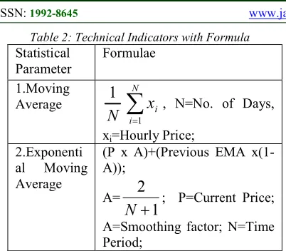
The Indian Rupee against US Dollar is taken as the experimental data. The total number of samples used is 9414, from 1st February 1973 to 16th July 2010. The used dataset is shown in Figure 3. Two important technical indicators, Moving Average and Exponential Moving Average are taken into consideration along with the exchange rate data. The used technical indicators and the formula are given in Table 2. In this model data are scaled between 0 and +1 as all the samples are divided by the maximum input value of the dataset. Scaling is not mandatory but it will help to improve the performance. The data is distributed into two, one dataset for training and the other for testing.
Fig. 3 Normalized Exchange Rate Data 0 2000 4000 6000 8000 0 0.2 0.4 0.6 0.8 1 Days E x c h a n g e R a te
Table 2: Technical Indicators with Formula
Statistical Parameter
Formulae
1.Moving Average
N
1
∑
=
N
i i
x
1
, N=No. of Days,
xi=Hourly Price;
2.Exponenti al Moving Average
(P x A)+(Previous EMA x(1-A));
A=
1
2
+
N
; P=Current Price; A=Smoothing factor; N=Time Period;The Mean Absolute Percentage Error (MAPE) and Root Mean Square Error (RMSE) are used to measure the performance of both LLWNN and MLP models. The MAPE and RMSE are defined as
MAPE=
1
ˆ
100
1
Χ
−
∑
=
N
i i
i i
y
y
y
N
(26)RSME=
(
)
2
1
ˆ
1
∑
=
−
N
i
i
i
y
y
N
(27)where yi isthe predicted value and
y
ˆ
i is the desiredvalue. N is the total number of test data. Gradient descent algorithm is used to optimize the parameters of both the models. As LLWNN has given better results as compared to MLP model, the former is integrated with PSO to get more accurate results.
5. OBSERVED OUTPUT
Table 3 demonstrates the comparison of MAPE for all type of experiments taken in this paper.
Table 3. Comparison of MAPE during Testing
6. ANALYSIS OF OUTCOME
From the graphs and the tables given above, three observations can be made: (1) LLWNN model is producing better results as compared to the MLP model irrespective of any time horizon chosen out of the four, as discussed in the study. (2) The proposed LLWNN model when integrated with PSO, giving more accurate results then the traditional derivative based backpropagation learning algorithm. (3) Prediction accuracy is inversely proportional to time horizon: increase in time horizon shows decrease in prediction accuracy. Fig. 8 shows the convergence speed of all time horizons discussed in the study for Rupees Vs Dollar dataset.
7. SUMMARY AND CONCLUSION
This paper used an efficient hybrid forecasting model for the currency exchange time series data. Results of the experiments show that PSO based Local Linear Wavelet Neural Network model can forecast currency exchange rate time series data for one day, one month, six months and twelve months in advance. After comparing the result with other time series models like MLP, it is proved that PSO based LLWNN model is superior in terms prediction accuracy and convergence speed. MAPE obtained from LLWNN model indicates that it can be used as a feasible alternative for exchange rate prediction for all stake holders in currency exchange market.
REFERENCES
[1] J. Hann, N. Kamber, (2001) “Data mining concepts and techniques”. San Francisco; Morgan Kaufmann Publishers.
[2] Sira-Ramirez Herbertt, Colina-Morles Elizer, Rivas-echeverria Francklin: (2000) “Sliding Mode-based adaptive learning in dynamical filter-weights neurons”, International Journal of Control, Vol. 73, No. 8.
[3] Chen Yuehui,Yang Bo, Dong Jiwen: (2005) “Time Series Prediction using a local linear wavelet neural network”. Elsivier B.V.
[4] Majhi Banshidhar, Shalabi Hasan and Fathi Mowafak: (2005) “FLANN Based Forecasting of S&P 500 Index” Information Technology Journal.
[5] Emam Ahmed (2008) “Optimal Artificial Neural Network topology for Foreign Excgange Forecasting” ACM-SE, Auburn, AL, USA, 978-1-60558.
[6] Yuehui Chen, Xiaohui Dong, Yaou Zaho (2005) “ Stock Index Modeling using EDA Model MAPE
(1 day ahead)
MAPE (1 month ahead)
MAPE (6 months ahead)
MAPE (12 months ahead) MLP 2.68 3.05 3.93 5.93
LLWNN 1.23 2.33 2.94 3.67
PSO based LLWNN
based Local Linear Wavelet Neural Network”
IEEE, 0-7803-9422.
[7] Chen Y H (2000) “Evolving the wavelet neural networks for system identification”- Proceeding of international conference on electrical Engineering.
[8] Ravichandran. K.S., Thirunavukarasu P., Nallaswamy R. and Babu R. (2005): “Estimation on Return on Investment in share market through ANN”, Journal of Theoretical and Applied Information Technology.
[9] Naeini Mahdi Pakdaman, Taremian Hamidreza and Hashemi Homa Baradaran, “Stock Market Value Prediction Using Neural Networks”, IEEE 978-1-4244-7818, 2010.
[10]Majhi Banshidhar, Shalabi Hasan and Fathi Mowafak, “FLAN Based Forecasting of S&P 500 Index” Information Technology Journal, 4(3): 289-292, Asian Network for Scientific Information 2005.