ISSN: 1992-8645 www.jatit.org E-ISSN: 1817-3195
VELOCITY INTEGRATION BASED PIPELINE
MAINTENANCE USING WSN
1,2ABDULAZIZ S. ALMAZYAD, 1QIANG MA
1
Department of Computer Engineering, CCIS, King Saud University, Riyadh, Saudi Arabia
2
College of Computer and Information Sciences, Al-Yamamah University, Riyadh, KSA Email:
[email protected], [email protected]
ABSTRACT
Pipeline is used worldwide daily to transfer liquid. This process covers large area and may pass through inhospitable environment and face many accidents such as leakage causing lose of resources and may cause hazards. It is necessary to monitor the pipeline system in order to prevent the waste from leakage, and at the same time to calculate the accurate location of the leakage so that it will be easy to maintain under the hot weather especially in desert. Thus we propose this new algorithm called Velocity Integration Method (VIM) for locating of the leakage. This method is easy to implement with lower cost and with high accuracy comparing to other approaches currently exist.
Keywords:Pipeline, Leakage, Solar Unit, Velocity Integration Method (VIM), Trapezoidal Area Method
1. INTRODUCTION
Our daily life depends on many types of pipeline to transfer and deliver liquid such as water, oil etc. According to a World Bank study [1], the worldwide losses of water due to the leakage is estimated approximately 14.6 billion US dollars per year, the leakage detection is considered to be one of the most serious challenges. Active monitoring and inspection is required to maintain the health of the pipelines [2, 3]. The leakage detection system has many tasks such as detecting and localizing leakage, monitoring flow speed [4, 5]. In many situation of transmission, pipeline covers large area and sometimes passes through inhospitable environment and it may face many accidents such as leakage, thieving etc. These accidents not only cause losing resources but also may cause hazards. In some countries, water is more precious than oil, so it is necessary to monitor the water pipeline system in order to prevent the waste from leakage. There are many techniques listed in the literature that have been developed over the past years to detect and calculate the location of leakage on pipes and investigate the status of pipeline network in transferring water, oil etc.
The rest of the paper is organized as follows: related work is discussed in Section 2, and Section 3 will present and discuss our model, then we explain the new algorithm in Section 4. Simulation results are discussed in Section 5 and then the conclusions will be given at Section 6.
2. RELATED WORK
A mobile sensor system dedicated for mapping water pipeline which is hidden inside cement wall or under floor coverings was proposed in [6]. This system works by dropping a small size sensor into the source of water pipelines. The sensor will traverse the pipeline and gather accelerometer and water pressure. In [7], pipeline leakage is detected and located by attaching vibration sensors to the pipe surface. Their system was examined and showed that vibration based on water flow rate estimation is feasible and the achieved individual per pipe flow rate error on average is less than 10 percent. In addition, an acoustic and vibration sensor was designed for monitoring water flow and detecting leaks in [8], it provided a number of useful properties including automated detection of leaks and bursts in water transmission pipelines. It is possible to carry out the analysis and data reduction in a real-time; consequently the storage and power consumption will be reduced. A leak-detection system which may minimize public risk of economic loss and conserve water was surveyed in [9], in order to determine the exact location of leaks by using acoustic listening devices and modern leak noise correlation, the authors mentioned that an acoustic equipment is more effective for metal pipes. In [10], where the author presented an initial framework using linear WSN for oil, and water pipeline monitoring.
ISSN: 1992-8645 www.jatit.org E-ISSN: 1817-3195 method to fill the gap. We use two kinds of sensors,
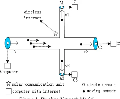
which are stable sensor to detect flow speed, and waterproof mobile sensor to detect leaks as shown in Figure 1.
3. MODEL INSTRUCTION
[image:2.612.95.294.274.438.2]In our model, we mainly focus on localization of leakage, while ignoring the detection techniques. We should consider the energy consumption at the beginning, in order to decide the sensors deployment strategy. Whether to use solar units or not, we need to decide the number of pieces and their locations in advance. The following Figure 1 is the model of our pipeline system.
Figure 1. Pipeline Network Model
Depending on the number of branches, we will decide the number of stable sensors to deploy at source and destination of each branch. These stable sensors will communicate with computer which has internet connection. In this model, we collect data from stable sensors at the source and destination to detect the speed of the flow. At time t=0, we deploy a number of mobile waterproof sensors, then the start time of this group of sensors will be 0. Each sensor records leakage information inside itself using in a list during its flowing. The structure of information list is shown in Figure 2.
[image:2.612.155.223.600.676.2]
Figure 2.Leakage Information List Structure
Strategy of recording leakage information: whenever the mobile sensor detects the leakage during its flowing, it will use a simple time-counter
to write down the time in its memory. The start time is the time of its deployment. The sensor will be switched on at a certain batch according to its tag, its information is read by solar communication unit to make sure the relay race goes smoothly without gaps among different batches.
When these mobile sensors move to solar communication unit, they will send their information including start time, and leak time list to the unit, after that they will delete the leak time list which has been sent out. Solar unit will send this information to internet through GSM. At the destinations people will collect all the moving sensors, recharge them and return to the source, get ready to reuse them for the next turn.
3.1 Assumptions
a. Long distance pipes system includes main pipe and branches, as shown in Figure 1, the main pipe is divided into three branches.
b. Single sensor continues sensing without sleeping in time t, so at the same time we have to deploy T/t sensors. T is the whole time of the liquid flowing from source to the farthest destination. Sleeping sensors will be switched on to start sensing just like a relay race. Also, we have to consider the branches, with the assumption that each branch will have a same probability, which means holding 1/3 quantity of the mobile sensors in its branch. So we should deploy at least 3T/t sensors at the source to make sure that all branches have enough mobile sensors.
c. Two main functions within the communication unit: Firstly it can communicate with passing by mobile sensors, to collect leakage information and send to internet using GSM to achieve the real time response. The unit is solar powered, so it is easy to use and without maintenance. Secondly it has to calculate using the sensing time ‘t’, and the minimum speed of liquid ‘v’. The distance interval should be less than v×t, to make sure the remaining energy of mobile sensors is enough for communication during their cycle. Thirdly these communication units are used for switching on the mobile sensors. If we assume that the mobile sensor can sense 100 hours, then it will not be exhausted during its travelling therefore the third function of the communication unit will be useless.
3.2 Basic Theory We Have To Use
ISSN: 1992-8645 www.jatit.org E-ISSN: 1817-3195 from t1 to t2, the water flowing speed is stable,
which means the water level is flat namely the water area “A” inside the section of pipeline keeps as a stable value, then we get a conclusion that in a short time duration, the water flowing speed is equal inside the pipe, as shown in Figure 3, the flowing speed keeps the value of “V” .
Figure 3. Speed Within Single Pipeline
b. According to Figure 1, at the time of t1, we
have the following equations based on physics. We assume that in a short time duration from time t1 to t2 the water flowing speed is stable.
Let V denote the water flowing speed at the source, Vi denote the water flowing speed of
branch i, A denote the water area inside the pipeline at the source and Ai denote the water
area inside the branch i. 2
1 t
in t
V A d t
Φ =
∫
(1)2
1
3
1
( )
t
o u t i i
i t
V A d t
=
Φ =
∑ ∫
(2)Φin = Φo u t (3)
4. PROPOSED ALGORITHM
Velocity Integration Based Location Algorithm a: The length of main pipeline → d.
b: To sense the water flowing velocity at source and each destination, adopting suitable sampling frequency, to get real time Figures vsource-t and vbranchi-t (i=1,2…n), and forward
this information to internet to make combined calculation.
c: To collect start time tstart and leakage sensed
time tleak,using Trapezoidal Area Integration
Method to acumulate.
d: If (tcumulate exists in Figure vsource-t) & ( tstart <
tcumulate < tleak ) then
If S(tstart-tcumulate)=d then l=S(tcumulate - tleak)
//cumulate using Figure vbranchi-t
return(d+l)
Else l= S(tstart- tleak)
// cumulate using Figure vsource-t
return(l)
End if End if
5. SIMULATION AND ANALYSIS
The main issue in our model is to fix the leakage
location. So we will focus on this part. Based on
our assumption, the energy is guaranteed.
5.1 Simulation Scenario
a. The length of main pipeline is 1000 km, and it connects with 3 branch-pipelines whose lengths are 500 km. So the length from source to each destination is 1500 km.
b. Single sensor can sense 100 hours above (energy is guaranteed).
c. We assume the range of flowing speed at source is [5,10] m/s, it equals to [18,36] km/h, and in order to simplify the calculation, we may set the flowing speed at destination of the branch as a constant, which is 7.5 m/s, equals to 27 km/h. So around [47, 75] hours a sensor may flow through the whole pipelines.
d. Considering the Fourier Transform, for each time-based signal can be expressed as an accumulation of different “Sin” signal, we may use Sin function to describe the flowing velocity of the source. To avoid influence of calculation accuracy within Matlab, we use constant value as flowing speed of destination in the branch.
e. To choose 3 points as leakages, they are Point A (in main pipe): 500 km far from the source, Point B (in main pipe): 1000 km far from the source, and Point C (in branch 1): 1200 km far from the source respectively.
f. At the time t=0, we deploy a group of mobile sensors, so that the start time should be 0. What we get from stable sensor are the samples of flowing speed at each dt instant, and what we get from the moving sensors are the start times and leakage information lists. We use Matlab to do the simulation and assume real flowing speeds etc as following:
9sin( ) 27
source
v = t + (km/h) (4) In time cycle: source speed=2×pi (hour) (5)
1 27
branch
v = (km/h) (6) We get Figure 4 for (4) and Figure 5 for (6).
ISSN: 1992-8645 www.jatit.org E-ISSN: 1817-3195
Figure 5. vbranch1-t
5.2 Simulation
Now we are going to set 3 points for our experiments.
Point A: 500 km
0
(9sin( ) 27) 500 leak
t
t + dt=
∫
(7)
To solve this equation we get the real leakage sensing time: tleak=18.4981(h) (8)
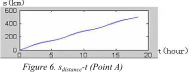
At source, we collect samples from stable sensor and use the Trapezoidal Area Method (TAM) to calculate the distance. If dt=0.1 hour, it means every 360 seconds we have to collect data from stable sensor. In our model we have set the frequency and range of flowing speed, so even 1 second error, we may have from 5 to 10 meters error. So we set dt=0.001 (hour) namely every 3.6 seconds we will collect the speed information from stable sensor, then by using TAM, the distance will be: Sleak=499.9965(km) (9)
as shown in Figure 6. Comparing to real distance 500 km, it is less than 4 meters’ error which is acceptable and efficient.
Figure 6. sdistance-t (Point A)
Point B: 1000 km
Similar like point A, we just show whether the time interval dt=0.001 hour is acceptable or not for a long distance.
0
(9sin( ) 27) 1000
leak
t
t + dt=
∫
(10)
To solve this equation we get:
tleak=36.9472 (h)
(11)
By using TAM we have:
Sleak=999.9968 (km) (12)
[image:4.612.108.297.461.534.2]as shown in Figure 7. Comparing to 1000 km, it still less than 4 meters’ error which is acceptable and very accurate.
Figure 7. sdistance-t (Point B)
Point C: 1200 km=1000(main)+200(branch 1)
0
(9sin( ) 27) 1000
main t
t + dt=
∫
(13)tmain=36.94(h) (14)
Continuing we have 200 km in the branch 1, so we start to use the flowing speed of branch 1:
27
tmain tleak
∫
dt=200 (15)Now the total time of the leakage detecting time is: tleak=44.3546 (h) (16)
We use TAM to calculate the distance. We still set dt=0.001 hour, since affected by calculation accuracy, the time which sensor flowing in main pipe will be a range from tcumulate1=36.945 (h) to
tcumulate2=36.949 (h), here we adopt average value as
our strategy. So we have:
tcumulate=36.947(h) (17)
then the estimated flowing time in branch will be: 44.3546 36.947 7.4076( ) remain leak cumulate
t =t −t = − = h
(18) Because time interval here is 0.001 hour, here we adopt a strategy to get a more accurate result applying in long distance case, so we use mean value 7.4075 as our estimated flowing time. Then we estimate the flowing distance in the branch, we get:
1 1 27 7.4075 200.0025( )
branch branch remain
s =v ×t = × = km (19)
Since we know the leakage is in branch 1, and the main pipeline is 1000 km, then our estimation of the total distance of the leakage will
be: 1
1000 200.0025 1200.0025( )
leak main branch
s
=
s
+
s
=
+
=
km
(20)
As shown in Figures 8&9.
ISSN: 1992-8645 www.jatit.org E-ISSN: 1817-3195
Figure 9. sdistance-t (Point C-part 2)
Since for long distance case, we adopt few strategy to guarantee the accuracy, then comparing our estimation which is 1200.0025 km with real distance which is 1200 km, it is less than 3 meters’ error, which proves our strategy and TAM is effective and efficient.
The total deployment cost: total number of mobile sensors + total number of stable sensors + solar units + transportation (to return the mobile sensors).
Considering the speed of drops at the leakage, we assume 12 hours are acceptable to detect leakage, so that every 12 hours labors at the source should deploy a group of mobile sensors with initialized start time, tags etc.
6. CONCLUSION
From the simulation and based on our assumptions, when sampling frequency is suitable for a given velocity curve, we can get accurate leakage locations. Along with the technology development, a single sensor could detect its moving speed. Using Trapezoidal Area Integration Method to accumulate the distance, while without knowing the velocity curve of the flow, water level, and all situations within pipelines, the proposed method can still get a high efficient result. This method is easy to implement with lower cost. The key points of our paper are velocity integration using Trapezoidal Area Method to calculate the leakage location, and few strategies to guarantee the accuracy of calculation.
In future, we have to improve the structure or network of our model, and also look for new type of sensors, so that we may design lower power consuming and high accuracy method.
REFERENCES:
[1] Cataldo. A., Cannazza. G., Benedetto. E.D., Giaquinto. N, “A new method for detecting leaks in underground water pipelines”, IEEE
Sens. J, 2012, 12, 1660–1667.
[2] Almazyad, A. S., Seddiq. Y.M., Alotaibi. A.M., Al-nasheri. A.Y., BenSaleh M.S., Obeid A.M., and Qasim S.M, "A Proposed
Scalable Design and Simulation of Wireless Sensor Network-Based Long-Distance Water Pipeline Leakage Monitoring System." Sensors 14, no. 2 (2014): 3557-3577.
[3] Seddiq. Y.M., Alotaibi. A.M., Al-nasheri. A.Y., Almazyad. A.S., BenSaleh. M.S., Qasim. S.M, “Evaluation of Energy-Efficient Cooperative Scheme for Wireless Sensor Nodes used in Long Distance Water Pipeline Monitoring Systems”, Proceedings
of 5th International Con. on Computational
Intelligence, Communication Systems and
Networks (CiCSyn’2013), Spain, June 2013;
pp. 107–111.
[4] Yuanwei J. , Ali E, “Monitoring of Distributed Pipeline Systems by Wireless Sensor Networks”, Pro. of The 2008
IAJC-IJME International Con., ISBN
978-1-60643-379-9.
[5] D. N. Sinha, “Acoustic sensor for pipeline monitoring”, Technical report, no. LAUR-05-6025, Los Alamos National Laboratory, July 20, 2005.
[6] Yu-Chen Chang, “PipeProbe: Mapping Spatial Layout of Indoor Water Pipelines”,
Mobile Data Management: Systems,
Services and Middleware, 2009,10th
International Conference,
DOI:10.1109/MDM.2009.69
[7] Y. Kim, T. Schmid, Z. M.Charbiwala, J. Friedman, and M. B. Srivastava, “NAWMS: Nonintrusive Autonomous Water Monitoring System”, Pro. of the 6th ACM Conference on Embedded Network Sensor
Systems, 2008, pp. 309–322.
[8] I. Stoianov, L. Nachman, S. Madden, T. Tokmouline, and M. Csail, “PIPENET: A Wireless Sensor Network for Pipeline Monitoring”, Proceedings of the 6th IPSN, 2007, pp. 264–273
[9] Hunaidi, O. Chu, W.T., Wang. A., and W. Guan, “Detecting leaks in plastic water distribution pipes”, Journal of the American
Water Works Association, 92 (2), 2000.
[10] Jawhar. I., Mohamed. N., Shuaib. K, “A Framework for Pipeline Infrastructure Monitoring Using Wireless Sensor Networks”, Proceedings of the Wireless
Telecommunications Symposium (WTS’07),