SRC Technical Note
1997 - 011
June 17, 1997
Tight Thresholds for The Pure Literal Rule
Michael Mitzenmacher
d i g i t a l
Systems Research Center130 Lytton Avenue Palo Alto, California 94301
http://www.research.digital.com/SRC/
Abstract
We consider the threshold for the solvability of random k-SAT formulas (for k≥3) using the pure literal rule. We demonstrate how this threshold can be found by using differential equations to determine the appropriate limiting behavior of the pure literal rule.
1
Introduction
We consider the problem of the performance of the pure literal rule in solving a random k-CNF satisfiability problem for k≥3.
The probability spacek
m,n is the set of all formulas in conjunctive
nor-mal form in n variables with m clauses each containing k literals. For exam-ple, the following formula is a member of2
4,3:
(x1∨ ¯x2)∧(x3∨x2)∧(x2∨ ¯x3)∧(x¯1∨ ¯x3).
When we speak of a random formula, or more specifically of random k-CNF formula with m clauses and n variables, we shall mean a formula chosen uniformly at random fromk
m,n. Note that an alternative way of thinking of
such a formula is that we randomly fill each of the mk “holes” with one of the 2n literals, each chosen independently and uniformly at random.
The pure literal rule is a heuristic for satisfying a CNF formula that works as follows. A pure literal is one whose complement does not appear in the formula (note that a literal and its complement can both be pure, in our un-derstanding). As long as there is a pure literal available, set a pure literal to the value 1 (true), remove all clauses containing that literal, and continue. The pure literal rule is the most conservative strategy, in that it only assigns a value to a variable that will obviously maintain the satisfiability of the for-mula.
Threshold behavior for the pure literal rule has been studied by Broder, Frieze, and Upfal [1], who found that for sufficiently large n a random 3-CNF formula with (approximately) 1.63n clauses can be solved by the pure literal rule with high probability, and a random 3-CNF formula with 1.7n clauses is not solvable by the pure literal rule with high probability. We expand upon their work here by finding an exact threshold by considering the limiting behavior as n → ∞using differential equations. These equations can also be thought of as describing the expected behavior of the system for large finite values of n. (For more on this approach, see also for example [3, 4, 5, 6, 7, 8].) The question of the performance of the pure literal rule is related to the more general question of finding thresholds for the satisfiability of random k-SAT formulas; see, for example, [2].
is not fully clarified, although it is easily checked using arguments from [1] and [4] or [8], for example. A full version to be prepared in conjunction with the authors of [1] will provide more complete details.
2
The Equations
We shall think of the pure literal rule in the following manner: at each time step, if there is a pure literal available, a pure literal is chosen uniformly at random from all pure literals. That literal and its negation are then deleted (removed from consideration), and all the clauses containing the pure literal are deleted.
In the following, all the variables are scaled by a factor of n, the number of variables in the formula. This is useful in writing the appropriate differen-tial equations. Hence (as will be seen below) if we inidifferen-tially have 10n clauses, we will represent this by a variable with value 10.
We shall describe the pure literal rule as a process running from time 0 to 1. The variables we shall use are functions of time described as follows:
• L(t): the scaled number of undeleted literals remaining
• Xi(t): the scaled number of undeleted literals appearing i times in the formula
• C(t): the scaled number of clauses; that is, the number of clauses remaining divided by n
• A(t): the average number of clauses in which a literal chosen uni-formly at random from all literals appears
We may drop the explicit dependence on t when the meaning is clear. Note that X0(t)is the scaled number of pure literals at time t . If X0(t)=
0 while C(t) >0, then the pure literal rule fails to find a solution; the pure literals have run out while clauses still remain. If, however, X0 goes to 0
only as C goes to 0 (and necessarily as t goes to 1), then the pure literal rule will succeed on a random formula with high probability. Hence our goal is to determine how X0behaves as we vary the ratio m/n. In particular, we shall
show that for some constant ck, X0stays above 0 on the interval t ∈[0,1)if
m/n<ckand it falls below 0 for some t<1 if m/n>ck.
We shall now determine equations that describe the limiting behavior as
n → ∞and m/n is held fixed. The initial values for C and Xi are easily determined: C(0) = m
n and, lettingµ = mk
n , Xi(0) =
e−µµi
i! , since in the
limit as n goes to infinity, the distribution of the number of times a literal approaches the Poisson distribution.
To set up the differential equations, we assume for each block of time dt (which can be though of as 1/n) we choose a pure literal uniformly at random
and remove it and its negation. Note that this assumes that X0(t) >0, and
the differential equations do not hold once X0(t)≤ 0. In fact when X0 =0
It is clear that d L
dt = −2, since at each step, two literals are removed.
Hence, as L0=2, we have L=2−2t .
When a random pure literal is chosen, the expected number of times it appears in the formula is simply the average number of clauses a ran-dom variable appears in (up to an O(1n)additive error). One can see this by noting that any given pure literal is equally likely to be any of the re-maining variables; the fact that its negation appears 0 times does not affect the conditional distribution of its number of appearances, given the current state(X0(t),X1(t), . . .). (The O(n1)discrepancy is caused by the fact that a
pure literal is slightly less likely that a random literal to appear 0 times, as we know that one literal, its negation, appears 0 times; this, however, only changes things by an O(n1)term, which can be safely dismissed in the limit as n → ∞. From now on, we ignore this discrepancy in establishing the differential equations.) Hence
dC
dt = −A= −
P
i≥0i Xi
L .
Making use of the identity Ck = Pi≥0i Xi, which expresses the total
number of remaining variables in the formula in two different ways, and our knowledge of the form of L , we may rewrite this as
dC
dt = − Ck
2−2t,
from which it is easily derived that C=C0(1−t)k/2.
The equations describing the behavior of the Xi are slightly more
com-plex. First, note that the pure literal deleted during a time step appears i times with probability Xi
L. Now, suppose the pure literal occurs j times. Then we
lose a literal that appears i times whenever one of j clauses containing that variable contains a literal that appears exactly i times. Note that there are
j(k−1)variables deleted, as there are k−1 variables per clause (1 variable for each clause is taken by the pure literal!). The probability that each such variable is one that appears i times is i Xi
Ck. (Again, note that we have here
ignored additive O(n1)terms, such as when a two appearances of a literal are deleted.) Hence the expected loss of literals of size i is−Xi
L − Ai Xi
Ck . One
can similarly determine the expected gain in Xi during a time step from all
literals that appear i+1 times and have 1 appearance deleted. The result yields:
d Xi dt = −
A(k−1)i Xi Ck +
A(k−1)(i+1)Xi+1
Ck −
Xi
L for i≥1.
Note the case of X0is special, since we always remove the negation of a
pure literal, which by definition appears 0 times, at each step:
d X0
dt =
A(k−1)X1
Ck − X0
3
The Solution
Recall that, once X0 =0, the process stops. Hence our goal is to determine
an explicit equation for X0, and use it to determine what values of m
guar-antee that X0 > 0 for t ∈ [0,1). Once we have solved this deterministic
case given by the differential equations, we can use this information to make statements regarding the limiting case of the random process as n → ∞. (Note that, for technical reasons, we also require k ≥ 3; see Lemma 4.4 of [1].)
For the equations below, we use c= mn which is a fixed constant. One may check that the solutions for the Xi, i ≥ 1, are given by the
following formulas:
Xi(t)=
∞
X
j=i
λi,j
C c
j(k−1)/k
(1−t)1/2,
where
λi,j =
2 ck2j(−1)i+j j i
j ! .
X0can be solved for explicitly, or by noting that X0=L−Pi≥1Xi, yielding
X0(t)=2−2t−
∞
X
i=1
∞
X
j=i
λi,j
C c
j(k−1)/k
(1−t)1/2.
We now find a convenient form for X0(t):
X0(t) = 2−2t−
∞
X
i=1
∞
X
j=i
λi,j
C c
j(k−1)/k
(1−t)1/2
= 2(1−t)1/2
"
(1−t)1/2−
∞
X
i=1
∞
X
j=i ck
2
j
(−1)i+j ij
j ! (1−t)
(k−1)j/2
#
= 2(1−t)1/2
(1−t)1/2−
∞
X
j=1
j
X
i=1
(−1)i+j
j i
!ck(1−t)(k−1)/2
2 j j !
= 2(1−t)1/2
(1−t)1/2+
∞
X
j=1
−ck(1−t)(k−1)/2
2 j j !
= 2(1−t)1/2
(1−t)1/2+exp
−(
1−t)(k−1)/2ck
2
−1
.
Hence, to determine when X0(t) >0, it suffices to examine the
expres-sion
(1−t)1/2+exp
−(1−t)(k−1)/2ck
2
and to determine the supremum of the set of all c such that this expression is positive for all t∈ [0,1). This can be found by finding the values of c and t such that the above expression is 0 at t and its derivative is 0 at t . This point must satisfy:
(1−t)1/2+exp
−(
1−t)(k−1)/2ck
2
−1 = 0
(1−t)−1/2
2 +exp
−(1−t)(k−1)/2ck
2
ck(k−1)
4 (1−t)
(k−3)/2 =
0
We use the first equation above to remove the exponential expression from the second by noting that it implies exp−(1−t)2(k−1)/2ck=1−(1−t)1/2
and substituting accordingly. The equations can then be solved for c to yield:
c= 2
k(k−1)[(1−t)(k−2)/2−(1−t)(k−1)/2].
This, in turn, yields a condition on t based solely on k:
(1−t)1/2+exp
−1
(k−1)((1−t)−1/2−1)
−1=0.
This can easily be solved numerically for the correct t ∈ [0,1)and in turn for the correct value of c.
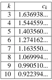
Using this framework, we derive Table 1 of values ck, where ck is the
appropriate threshold for k-SAT formula. That is, ckis the number such that
for any fixed > 0, if we have a random k-SAT formula with n variables and(ck−)n clauses, with high probability we may find a solution using the
pure literal rule, while if we have(ck+)n clauses with high probability the
pure literal rule fails to find a solution.
References
[1] A.Z. Broder and A. M. Frieze and E. Upfal. On the satisfiability and maximum satisfiability of random 3-CNFformulas. Journal of Algo-rithms 20 (1996) pp. 312–355.
[2] A.M. Frieze and S. Suen. Analysis of two simple heuristics on a random instance of k-SAT. InProceedings of the Fourth Annual ACM-SIAM Symposium on Discrete Algorithms (1993) pp. 322–330.
k ck
3 1.636938...
4 1.544559...
5 1.403560...
6 1.274162...
7 1.163550...
8 1.069994...
9 0.990510...
[image:7.612.262.348.69.200.2]10 0.922394...
Table 1: The thresholds for the pure literal rule for k-SAT. These values match simulations quite well even for a very small number of clauses (in the tens of thousands).
[4] R. M. Karp and M. Sipser. Maximum matchings in sparse random graphs. InProceedings of the 22nd IEEE Symposium on Foundations of Computer Science (1981) pp. 364–375.
[5] T. G. Kurtz. Approximation of Population Processes. SIAM (1981)
[6] M. Mitzenmacher. Load balancing and density dependent jump Markov processes. InProc. of the 37t h IEEE Symp. on Foundations of
Com-puter Science (1996) pp. 213–222.
[7] M. Mitzenmacher. The Power of Two Choices in Randomized Load Balancing Ph.D. thesis, University of California, Berkeley. (September 1996)