AUTOMATIC ITERATIVE OPERATION ON AN ANALOG COMPUTER
by
George Hannauer, Omri Serlin, and Peter J. Holsberg
Recent developments in analog computers have aroused fresh in-terest in automatic iterative computation. While the technique is not new, it has not been widely used with analog computers in the . past, and is therefore unfamiliar to many analog programmers. It is the purpose of this report to provide an introduction to the tech-niques involved and to suggest representative applications.
While the analog computer is, in many ways, well-suited for this mode of operation, many of the basic concepts (logical decision, storage, discrete variables) are more familiar to users of digital computers. Iterative analog computation is, in fact, a form of hy-brid computation, employing both analog and digital techniques, and large and complex iterative problems are most effectively at-tacked by combining digital devices (flip-flops, shift registers, gates, etc.) with conventional analog components. Nevertheless, a good many problems can be solved with analog components alone, and this report will deal almost exclusively with this type of prob-lem. Specifically, the report will be concerned with what can be done with existing components on a medium sized general purpose analog computer such as the PACE ® TR-48.
Of particular interest in this regard, however, is the hybrid imple-mentation (described in Appendix 3) of the illustrative analog problem solved in the body of the study. Using the EAI DES-3~
Digital Expansion System ... a general purpose, patchable digital logic package ... to provide digital expansion of the TR-48 analog computer, the all-analog simulation ofthis one-parameter optimizer or boundary value problem is modified so that the necessary logic functions are performed by the synchronous logic elements of this completely self-contained unit.
Although capable of operating autonomously as an aid to digital instruction or design, the DES-3~ digital logic system provides basic hybrid capabilities to the small computer facility. It is readily combined also with other general purpose analog or digital computers to provide extended control functions.
TABLE OF CONTENTS
Page
1. DEFINITION OF ITERATIVE COMPUTATION ••••• 3
2. TYPICAL APPLICATIONS •••••••••••••••••• 4
a) Parameter Sweep . . . • . . . • . . . • . . b) Optimization
c) Boundary-Value Problems •••••••••••••••
d) Curve-Fitting ••••••••••••••••••••••••
e) Serial Solution of Partial Differential Equations ••
3. ITERATIVE REQUIREMENTS AND CIRCUITS
4 4 4
5 5
USING ONLY ANALOG INTEGRATORS •••••••• 7
a) Storage . . . 7 b) Relay Logic ••••••••••.••••••••• ~ • • • • 9
c) Automatic Parameter Adjustment .••••••••• 9
d) Mode Control •••••••••••••••••••••••• 10
4. ITERATION SCHEMES . • • • • • • • • • • • • • • • • • • • . 12
a) Correction Proportional to Error • • • • • • • • • • • 12
b) Fixed~Step-Size Iteration •••.•••••••••••• 12
5. PROGRAM FOR ITERATIVE SOLUTION OF
BOUNDARY-VALUE PROBLEM USING ONLY ANALOG COMPONENTS:
(The Trajectory of a Bullet)
APPENDIX I
Parameter Sweep Circuit
APPENDIX II
TR-48 Relay Mode Control
APPENDIX III
- TR-48/DES-30 Hybrid Implem~ntation of One
14
18
19
Parameter Optimizer (Boundary Value Problem) 21
APPENDIX IV
AUTOMATIC ITERATIVE OPERATION
ON AN ANALOG COMPUTER
by
George Hannauer,
Omri Serlin, and
Peter J. Holsberg
1. DEFINITION OF ITERATIVE OPERATION
By iterative operation of an analog computer will be meant any sequence of operations that involves: (1) automatic cycling of the computer mode so that the computer goes through a number of OPERATE cycles, and (2) automatically changing some con-dition of the problem - an input, a parameter value, or an initial condition - between successive OPERA TE cycles so that a slightly different prob-lem is solved with each iteration(-::\ '
II
,.. " , ,,"-' /
i.,:,'"Th~
'second60h~ihon i~' importa~t.
It distinguishes true iterative operation from repetit~ve, operation, which satisfies only the first condition. Repetitive operation, in fact, is not a computational technique at all, but merely a form of readout, or display. No special techniques are involved in programming a rep-op problem; in fact, programming a problem is the same for rep-op as for "real time" read-out, with the exception that the programmer must restrict himself to high-speed components (e.g. quarter- square multipliers instead of servos).In repetitive operation, much of the information generated is redundant; except for occasional
manual parameter changes, the same problem is solved again and again, and the same curve gen-erated repeatedly. In contrast, each OPERATE cycle in iterative computation investigates a slightly different set of parameter values, and produces slightly different results. In a given number of cycles, therefore, iterative operation generates considerably more information, utilizing more fully and efficiently the analog computer's ability to produce a large amount of data in a short period of time.
\
j
\
,. 2. TYPICAL APPLICATIONS
a) Parameter Sweep. For a simple example of automatic iterative operation, consider the ef-fect of an adjustable parameter, '" , on an analog computer solution. It might be desirable to study the steady-state error of a position servo as a function of controller gain or some other control parameter, or the area of in-terest might be in the miss distance of a mis-sile as a function of initial launching error.
In either case, prime interest is in a single number, X, (steady-state error, miss distance, etc.) which is computed during an OPERATE cycle using a particular value of some param-eter, '" (controller gain, launching error, etc.). A value of·", is chosen at the beginning of the OPERATE cycle, and the corresponding value of X is computed (usually X will be a final value, i.e. the output of some component atthe end of the OPERATE cycle). It is desired to obtain a plot of X versus "'.
Obtaining such a plot manually can be quite time-consuming. The operator has to choose several values of "', changing pots manually between runs and tabulating the result X after each run. He can then make a point-plot of X versus '" and connect the points by a smooth curve. The procedure outlined below replaces this tedious work with a single computer run, in which the desired graph is automatically produced by an X- Y plotter. The necessary circuit is described in Appendix 1.
b) Optimization. Optimization problems arise quite frequently in design studies. In many cases, a long sequence of computer runs is made, with parameter adjustments between runs to achieve some optimum condition such as maximum profit, minimum cost, minimum error, etc.
For example, consider the design of a control system to stabilize the orientation of a satellite. Suppose the system is characterized by two parameters: a gain K and a dead-zone d. The problem is to correctagivenorientatio;-error with minimum fuel consumption. The general approach is given in Figure 2-1.
The computer is placed in the OPERATE mode for a sufficient length of time to correct the initial error, and the amount of fuel used is "remembered" by a storage device. The values of X from several successive OPERATE cycles may be stored if needed. On the basis of these
K
CIRCUIT FOR SOLVING
EQUATIONS OF MOTION X
d OF THE SATELLITE
CONTROL CIRCUITRY
:-.- I) RESET COMPUTER, BUT STORE
THE VALUE OF X OBTAINED IN COMPUTATION.
2) CALCULATE CHANGES IN K
4-AND/OR d TO DECREASE X.
3) OPERATE COMPUTER WITH
NEW PARAMETER VALUES.
4) REPEAT STEPS 1-3.
d = WIDTH OF DEADZONE IN ERROR SENSING DEVICE
K = CONTROLLER GAIN
X = AMOUNT OF FUEL USED IN THE CORRECTING
MANEUVER
Fiaure 2-1
results, changes are made in d or K or both, and the problem is re-run. The process is continued until a minimum is reached.
This type of problem differs from parameter sweep in that the former is purely "open-loop" Le. the changes in parameter values are determined in advance, while in optimiza-tion problems the parameter changes are allowed to depend on the results of previous runs. The circuitry for performing the re-quired storage, parameter changes, etc. will be discussed in Sections 3 and 4.
c) Boundary-Value Problems. The analog com-puter is essentially an initial-value device; that
is, from the many possible solutions to a given set of differential equations, a single one is de-termined by specifying initial values for the variables, Le, values at time zero, In contrast, many problems are stated in terms of boundary values, which must be met by trial and error, Le. by some sort (If iteration nrocess.
The most common examples of boundary value problems arise in the solution of partial dif-ferential equations which are discussed below. However, occasionally one runs into the same problem with ordinary differential equations, as in the following example:
velocity Vo. In the absence of air resistance, the trajectory of the bullet is described by the equations:
x
=Vo cose x(o) =0 (2-1)y
=-g y(o) = 0; y(o) = V 0 sin e (2-2)where x and yare the horizontal and vertical coordinates of the bullet respectively, as in Figure 2-2.
y
---f--~---~--~~
Figure 2-2
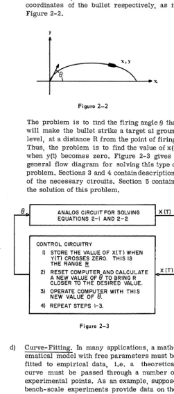
The problem is to tind the firing angle e that will make the bullet strike a target at ground level, at a distance R from the point of firing. Thus, the problem is to find the value of x(t) when y(t) becomes zero. Figure 2-3 gives a general flow diagram for solving this type of problem. Sections 3 and 4 contain descriptions of the necessary circuits. Section 5 contains the solution of this problem.
~
ANALOG CIRCUIT FOR SOLVING X(T)EQUATIONS 2-1 AND 2-2
CONTROL CIRCUITRY
IJ STORE THE VALUE OF X(Tl WHEN
Y(T) CROSSES ZERO. THIS IS THE RANGE B.
' - - 2) RESET COMPUTER AND CALCULATE A NEW VALUE OF 8 TO BRING R
xm
CLOSER TO THE DESIRED VALUE.
3) OPERATE COMPUeER WITH THIS
NEW VALUE OF .
4) REPEAT STEPS 1-3.
Figure 2-3
d) Curve-Fitting. In many applications, a math-ematical model with free parameters must be fitted to empirical data, i.e. a theoretical curve must be passed through a number of experimental points. As an example, suppose bench-scale experiments provide data on the decomposition of a component in a chemical reaction. Chemical theory and/or experience
suggest that the decay should satisfy the dif-ferential equation.
(2-3)
where C (t) is the concentration of the chemi-cal at time t. The problem is to find numeri-cal values of k and n so as to provide the closest agreement between the theoretical curve and the experimental data.
Let C(t) be the solution to the equation (with given values of k and n) and C*(t) be the ex-perimental curve. Then, it is desired to choose k and n so as to make C(t) and C*(t) as close as possible.
To automate this, it is necessary to define some measure of the error. Defining
€ =
f
[c
(t) - C* (t)] 2dt (2-4)the computer can be programmed to make E as small as possible. Thus, curve-fitting prob-lems can be treated as a special case of opti-mization problems.
e) Serial Solution of Partial Differential Equa-tions. The solution of partial differential equations on a general-purpose analog com-puter by the usual finite-difference techniques involves a large number. of similar circuits operating simultaneously. If the mesh size is small or the number of independent variables is large, then the duplication of equipment may make this approach prohibitively expensive. The simularity of circuits leads to the idea of using a single "time-shared" circuit; that is, a single circuit which performs sequen-tially the calculations that would otherwise· be performed Simultaneously by many similar circuits.
Consider the heat equation
K
with boundary conditions
aT
at
T (0, t) =f (t)
T (L, t) = g (t)
T (x, 0) =h (x)
(2-5)
[image:5.629.50.302.166.733.2]rod of length L with an initial temperature distribution h(x) and time-varying tempera-tures f(t) and g(t) established at the ends.
The usual approach to analog solution of this problem is to treat x as a discrete variable, replace partial derivatives with respect to x by finite-difference approximations, and solve the resulting ordinary differential equations in the conventional manner.
For serial solution, the best approach is to treat t as a discrete variable and work with a system of ordinary differential equations in x. tII.tIie···
...r.eaderc .. doubts·this,
he
fuayattempt serial solution with· discrete x 'and continuous t and struggle with Jhe boundary conditions;)Replacing the time-derivatives with finite-difference approximations, the following equation is obtained:
Til (x, t) + K T (x, t) - T (x, t - At) (2-6) At
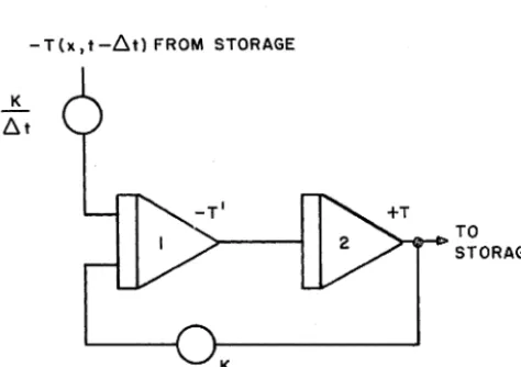
where T', T" refer to derivates with respect to x (not t). Since the integrators on an analog com-puter integrate with respect to time, it is necessary to represent distance in the heat equation by time on the machine. The circuit for solving equation 2-6 is given in Figure 2-4.
-T(x,t-6.tl FROM STORAGE
K
6.t
TO STORAGE
Figure 2-4. Circuit for Solvinq Equation 2-6
The fact that computer time represents distance in the original equation must be taken into account in interpreting the results.
The length of the OPERATE cycle is proportional to the length of the rod. The graph produced by the
computer during a single OPERATE cycle is an instantaneous temperature profile. Establishing boundary values T (o,t) and T (L,t) for T at both ends of the rod means establishing initial and final values for the output of integrator 2.
Establishing the initial value is no problem since this means putting an initial condition directly on integrator #2. To establish a final value, an ap-propriate initial condition must be picked for integrator #1. This requires an iterative procedure similar to the one used for the missile trajectory problem described above. The sequence of steps would be as follows:
1) Use the circuit in Figure 2-4 to calculate T(x, Ll t) with the given function h(x) =
T(x,o) as an input. Use f(Ll t) = T(o,Llt) as an initial condition on amplifier 2, and guess at an initial condition for amplifier 1.
2) At the end of the OPERATE cycle, com-pare the final value T (L, At) with the de-sired value g( Ll t), and change the IC on amplifier #1 accordingly.
3) Iterate until the condition T(L, Ll t) = g( Ll t) is met.
4) When this condition is met, store the com-plete curve T(x, Ll t) and repeat steps 1 - 3
with T(x, Llt) as an input to generate T(x, 2 Ll t).
Continuing in this manner, a sequence of temp-erature profiles is obtained: T(x, 0) (given), T(x, Ll t), T(x, 2 Ll t) . . . . T(x, n Llt).
NOTE that this application involves an iteration within an iteration. Such computations are referred to as nested computations.
All of these problems, with the
po~~'~hle
exception of the last, can be solved on the TR-48 provided the number of adjustable parameters involved is not too great. What distinguishes the last example is the need for curve storage - the entire curve T(x, At) must be stored and used as an input to generate T(x, t + Llt) in the next OPERATE cycle. In contrast, only a few numbers need be remem-bered at anyone time to solve the other problems." " i I I"
[image:6.630.55.292.463.630.2]3. ITERATIVE REQUIREMENTS AND CIRCUITS USING ONLY ANALOG INTEGRATORS
In each of the preceding applications the conven-tional analog circuit that solves the dynamic equa-tions of the basic problem is supplemented by a number of additional components to perform the iteration. These additional components must be capable of performing the following functions:
Storage: The computer must "remember" the results of previous computations, using them, if necessary, in the computation of new parameter values for successive runs.
LogiC: The computer must decide which pa-rameter(s) to alter, and must route signals into and out of storage in response to the re-sults of past computations.
Automatic Parameter Adjustment: The com-puter must be able to change the values of important parameters and initial conditions.
Mode Control: The computer must be auto-matically cycled through a sequence of modes. Normally, the RESET and OPERATE modes will alternate, but more complicated sequences are sometimes desirable.
The ability of a computer to store information, make logical decisions, and alter its own program has long been a familiar concept to digital com-puter users. What is not so well known is that an analog computer can also perform these functions, as the following pages will indicate.
This section will deal with the above requirements and how they can be met on an analog computer. The circuits given below are not necessarily the best or most economical. They have been chosen with one overriding consideration in mind - they can be mechanized by ordinary general-purpose analog components, without special-purpose ex-ternal equipment.
a) Storage. Since an analog signal is a voltage, it may be stored on a charged capacitor. Read-out of the stored information must take place without drawing appreciable current from the capacitor, as drawing current will partially discharge it, resulting in an erroneous read-ing. This requirement for "nondestructive readout" impiies that an amplifier will be necessary.
Consider the circuit in Figure 3-1 in which an amplifier and a capacitor are combined. Were it
not for the presence of the capacitor, this circuit would simply be an inverter with the relation Vout =-Vin'
The effect of the capacitor is to make Vout lag slightly behind - Vin, but this lag will be negligible provided Vin is not changing too rapidly, and the capacitor is sufficiently small. (The transfer func-tion of the circuit is
Vout 1
Vin 1 + RSC
and this is nearly -1 as long as the time constant RC is small.)
If the relay is opened, the amplifier behaves like an integrator in the HOLD mode, and Vout remains constant at the value it had when the relay opened. The amplifier is said to track, or follow its input voltage when the relay is closed, and store, or hold its value when the relay is opened.
R R
c
Figure 3-1
The circuit in Figure 3-1 is essentially the initial condition circuit of an integrator. If an input vari-able is patched into the IC terminal of an integra-tor, the integrator will track that variable in the RESET mode and store it in the HOLD mode (and even in the OPERATE mode if the integrator has no other inputs).
INPUT
T
tC>
OUTPUTTRACKING AMPLIFIER
Patch RESET coil to OPERATE bus Patch OPERATE coil to RESET bus Remove
f3
plug(Tracks when computer is in OPERATE; stores when computer is in RESET)
INPUT
~
OUTPUTsV----STORAGE AMPLIFIER
Patch OPERA'rE and RESET coils normally Remove
f3
plug(Stores when computer is in OPERATE; tracks when computer is in RESET)
~--"';""-III
INPUT
OUTPUT
COMPARATOR CONTROLLED TRACK-STORE UNIT
Omit mode control connections
Connect SJ; (not SJ) to B through comparator contacts
(Stores when comparator is open, tracks when comparator is closed)
Remove
f3
plugNotes:
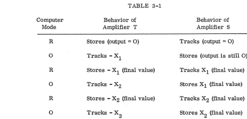
1) The T and S amplifiers are named after what they do in OPERATE - T tracks and S stores. In RESET, they do the opposite.
2) Input resistor networks need not be patched.
3) Removal of
f3
plug reduces the tracking error by shortening the time constant.In order to store a result from a previous compu-tation cycle, a tracking amplifier and a storage amplifier in cascade are used, as in Figure 3-2. The problem variable, X (t), is tracked during an OPERA TE cycle, and its final value is stored between OPERATE cycles .. The result is shown in Table 3-1; after every OPERATE cycle except the first, the output of amplifier S is the final value of X from the previous computer run. If it is desired to store a value of X other than a final value, the T amplifier can be replaced with a comparator-controlled track-store unit.
In OPERATE, T tracks and S stores. In RESET, their functions are reversed.
x
(t)T
Figure 3-2
Table 3-1 indicates the behavior of T and S ampli-fiers, where Xl, X2, X3 are the solutions produced during the 1st, 2nd, 3rd OPERATE cycle.
TABLE 3-1
Computer Mode
R
o
R
o
R
o
Behavior of Amplifier T
Stores (output = 0)
Tracks - Xl
Stores - Xl (final value)
Tracks - X2
stores - X2 (final value)
Tracks - X3
-Behavior of Amplifier S
Tracks (output
=
0)Stores (output is still 0)
Tracks Xl (final value)
stores Xl (final value)
Tracks X2 (final value)
[image:8.627.48.517.48.792.2] [image:8.627.67.483.546.747.2]b) Relay Logic. Logical decisions on the analog computer are often made by relay compara-tors. The relay comparator consists of a high-gain amplifier whose output drives the coil of a DPDT relay. The relay contacts normally make to the side marked "+"; they transfer to the side marked "-" when the sum of the input voltages becomes negative. (See Figure 3-3.)
x----..,
CIRCUIT SYMBOL
1 0
-~
1 0
-RI
~
X3J
C>
~
y R2 I--iIIG...--ILIMITER
~ ~ Rl~~Y
[image:9.613.357.513.219.318.2]SIMPLIFIED SCHEMATIC
Figure .3-3. The Relay Comparator
It should be noted that the input resistors on the TR-48 comparator are not equal. Therefore, a pot may be necessary to attenuate one of the inputs and assure that the switching occurs exactly when X + Y crosses zero.
The comparator is numbered with the number of the amplifier immediately to its left on the patch panel; this convention m~kes it easy to locate the com-parator when patching. The letters "U" and "L" on circuit diagrams refer to the upper and lower sets of contacts respectively.
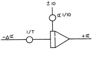
c) Automatic Parameter Adjustment. A param-eter in an analog computer circuit is a num-ber which is constant during any single OP-ERATE cycle, but which is allowed to change value between successive OPERATE cycles. Usually such parameters are represented by pot-settings, and the pots are adjusted man-ually between computations. However in auto-matic iterative computation, the
p~rameter
value is changed by the computer itself, which means that the parameter must be regarded as a computer variable, that is, as an ampli-fier output voltage.Let '" be the parameter that must be maintained constant during a computer run and vary between runs by an amount 11 "'. The value of 11"" i.e. the magnitude and direction of the change in "', can be made to depend on the results of previous com-putations. Hence, 11", will also be an amplifier out-put voltage. Methods of calculating 11", are dis-cussed in Section 4.
The easiest way to change '" in the desired manner is to use an integrator, as in Figure 3-4.
±IO
Figure 3-4
Since '" is to be constant during a computer run, the integrator must be in the HOLD mode when the rest of the computer is in the OPERATE mode. Since '" is supposed to change between computer runs, the integrator must be in the OPERA TE mode when the rest of the computer is in RESET and the problem is being reset for the next run. This type of mode behavior can be achieved on a TR-48 by patching the OPERATE coil to the RESET bus. (See Appendix 2 for an explanation of TR-48 mode control.)
If the computer resets for T seconds between OPERATE cycles, the integrator in Figure 3-4 will integrate the constant -l1o/T for T seconds, and its output will change by an amount 11 ",for the next computation.
An "initial condition" must be chosen for"" that is a value for the first run. This is, of course, an initial condition on the integrato:>'. The mode control must be arranged so that the integrator is in the RESET mode at the beginning of the iteration. A method of accomplishing this is given in Section 3d.
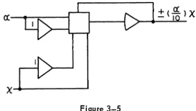
The three most common uses of the signal are:
1) as an initial condition
2) as an additive constant, or bias voltage
In cases 1) and 2) the voltage 0: may be fed directly
to the problem, as a voltage input is what is re-quired. In the third case, 0: exists as a voltage, but a coefficient is needed. This means that a quarter-square multiplier must be used, as shown below.
( ! - " ' t - - . : - - - ;
x ... ---'
Figure 3-5
The net result is that an input is multiplied by a constant coefficient, 0: /10, which is a number be-tween zero and one (in magnitude). This circuit is, therefore, equivalent to feeding x through apot, except that changing the value of 0: will "reset
the pot" automatically.
d) Mode Control. For the purposes of iterative computation, it is necessary to cycle the com-puter mode automatically between RESET and OPERATE. The repetitive operation unit does exactly this, and can be used in some forms of iterative computation. However, its use
suffers from a number of limitations:
1) For some purposes it is too fast - the longest OPERATE cycle obtainable is 200 milliseconds, which makes readout on an X- Y plotter impractical. Also, many pro-grams rely heavily on relay comparators to make the necessary logical decisions, and a 200 millisecond OPERATE cycle followed by a 10 millisecond RESET cycle does not always allow these relays suffi-Cient throwing time.
2) When using the rep-op drive, there is some uncertainty about the first and last cycles. Switching transients may destroy the accuracy of the first computation. In
"open-loop" iteration, (parameter sweep) this is not a serious defect, but in' 'closed loop" iteration, in which the parameter values for a given OPERATE cycle depend on the stored results from previous cycles, the effect can be serious.
3) It is desirable to have a means of cycling the computer mode on machines not equip-ped with rep-op.
The circuit below meets all these requirements. The RESET and OPERATE times are individually adjustable over a wide range. The iteration is started and stopped by a manual switch. This switch allows the entire iteration to be switched through RESET, HOLD, and OPERATE modes.
L
-20 VOLTS / . C
(RELAY SUPPLY) SI R
•
TO RESET COIL OF AOO TO OPERATE COl L OF AOO
TO RESET COl LS OF PROBLEM INTEGRATORS
TO OPERATE COILS OF
a PROBLEM INTEGRATORS
-10-0
+10
34U~
VII'11
Finally, this circuit, which involves only one inte-grator, two pots, and a comparator, can be used on machines not equipped for repetitive operation.
When using this form of relay switching, the indi-vidual integrator coils should be patched directly to the switch and relay contacts. The regular mode busses are not used.
Switch Sl is initially in the LEFT position putting ADO in RESET and all integrators which are patched to the relay contacts in HOLD.
Putting switch Sl to the CENTER position puts every integrator in HOLD. When Sl is thrown to the RIGHT position, ADO integrates and produces an asymmetrical sawtooth, as shown in Figure 3-6. ADO starts from an initial condition + lOa and integrates down at the rate of -lOb volts per second. When it reaches -10 volts, comparator 34 switches, and ADO integrates up at the rate of
+ 10ab volts per second until it reaches + lOa, when comparator 34 switches again. The integrators patched to the comparator contacts are cycled between RESET and OPERATE.
vet)
+100
[image:10.621.74.275.138.252.2]-100
The output of AOO varies from + lOa to -10 volts. The total voltage variation is lOa + 10 or 10 (a+ 1) volts. With Comparator 34 in the "+" position (which puts the computer on RESET) the rate of integration is -lOb volts per second, and hence if TR is the length of the RESET cycle the result is lOb TR = 10 (a+ 1) or
T = a + 1
R b
Similarly, the integration rate of AOO is + 10ab volts per second when comparator 34 is in the "-" position and the computer is in OPERATE. So, therefore, 10ab TO = 10 (a+ 1) or
T = a + 1
o
ab.where TO is the length of the OPERATE cycle.
Solving for a and b,
If a ten-second OPERATE cycle followed by a one-second RESET cycle is wanted, a =0.100 and b = 1.100 is necessary. Since apot-setting greater than 1 is impossible, a gain of 10 on the integrator is used and the "b" pot is set for bl10 = 0.110.
The operational procedure is as follows: put the manual switch to the left, and select the HOLD mode on the pushbutton mode-control panel. It
can be regarded that the L, C, and R switch posi-tions represent RESET, HOLD, and OPERATE cycles for the entire iteration; RESET and OPER-ATE for the individual runs are obtained by the switching of comparator 34.
In section 3C an integrator was used for automatic parameter adjustment. This integrator must cycle between HOLD and OPERATE during the iteration, but should be reset at the beginning of the itera-tion. This object can be achieved by patching its OPERA TE coil to the + contacts and its RESET coil to the left contact on the manual switch. The integrator will then be reset with AOO.
4. ITERATION SCHEMES
In cases where a parameter, oc, is being used to meet a boundary value or a minimum condition, it must be decided what change to make in oc for the next run. A formula for calculating the parameter value for the next run from the results of previous runs is called:an interation scheme. Two iteration schemes will be considered here. For simplicity, they will be limited to the case of a single param-eter, oc. Iteration with several parameters is con-sidered in References 6 and 7.
a) Correction Proportional to Error. Suppose it is necessary to vary a parameter or initial condition, oc, to meet the boundary condition Xf = a, where Xf is the final value of a variable X, such as the horizontal displacement of the bullet in the missile trajectory problem or the temperature T in the heat equation.
If an error is defined by ( =Xf - a, then a
reason-able change in oc would be
where G is a constant. This scheme makes large corrections for large errors and small corrections for small ones, which is reasonable. If oc eventually settles down to a steady value, thenflocwill approach zero, and therefore £ will approach zero, which is what is wanted. \\, l . , ' , : ' . ' , . \ \
,
If £ is an
increasi~g f~ction:
'of oc,tl~~n'
the con-' .lstant G should be negative so as to change oc in the right direction to decrease £. On the other hand, if £ is a decreasing function of oc, then G should be positive. This means that the method is most useful in cases where it is known a priori whether (.,':
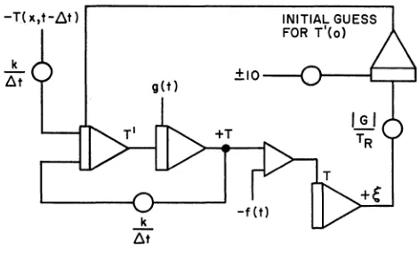
£ is increasing or decreasing with",. This is the case with the heat equation. Figure 4-1 shows how Figure 2-4 may be modified by adding storage and parameter change circuits to effect the iteration scheme. The parameter '" to be varied is oc = T (0)
and the computer effects the change in oc by inte-grating the error £ during the RESET cycle, whose length is TR.
In cases where £ is sometimes an
increasingfunc-tion of '" and sometimes decreasing, the above scheme is less practical. In these cases an alterna-tive is to minimize the absolute error
I
£ \. Thisapproach reduces the boundary value problem to a problem in optimization.
/ " . . . . "
l'l
~ " , ' , ' " !
b) E-med ... Step:,Si,ze Iteration. Consider theprob-lem of chOOSing a value for the parameter oc to minimize the result X. X may be the absolute
-T{x,t-Atl INITIAL GUESS
FOR T'{o)
k At
k At
[image:12.613.315.550.76.223.2]get) ±IO
Figure 4-1. Iterative Circuit for Solving the Boundary-Value Problem in Section 3e, Using the Iteration Scheme fl oc = Ge
" I
error in a boundary value problem, asdescrib-ed in Section 4a above, it may be the error in a curve fitting problem, as in Section 2d, or the amount of fuel consumed during a satellite maneuver, as in Section 2b. Many iteration schemes are possible, but the following one is probably the simplest to mechanize. (In
the following paragraph, subscripts refer to computer runs. Thus'" 1 is the value of oc used in the first run, Xl is the result obtained from the first run, etc.)
1) Pick a starting value for oc, say '" 1
2)
3)
Make a run with this value and store the result Xl
': '\ (
Change oc by a fixed amount fl oc and make a new run with the value oc 2 = oc1 + fl "'. Store the result X2.
! ( '
i \ . . ~ .
4)
5)
6)
Compare the values Xl and X2. If X2
<
Xl, increase oc by the ~ amount floc and repeat.Continue as long as X decreases with each successive change in '" .
When finally an increase in X is obtained this is an indication that the minimum value has been overshot. When this hap-pens, cut the step-size floc in half, and re-verse its sign.
Run #
x
/1", for next run1 1.00 +9.82 +1.00
2 2.00 +7.17 + 1.00
3 3.00 +6.61 + 1.00
4 4.00 + 6.29 + 1.00
5 5.00 +6.73 -0.50
6 4.50 +6.10 -0.50
7 4.00 + 6.29 +0.25
8 4.25 +6.07 +0.25
9 4.50 +6.10 -0.125
10 4.375 +6.02
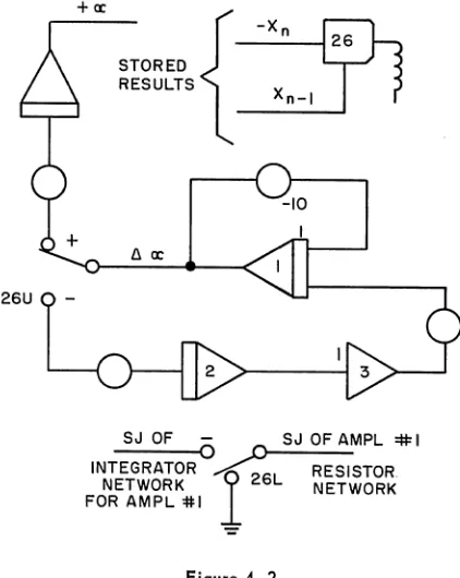
etc.---Note that some of the runs are redundant; run 7 duplicates run 4 and run 9 duplicates run 6, but this duplication is not a serious drawback. To mechanize the reversal of sign, the following cir-cuit can be used:
The mode control relays on integrators 1 and 2 are patched so that they integrate in RESET and hold in OPERATE. The comparator contacts assure that the integrators will receive inputs only when Xn> Xn-l; that is, only when the last parameter change made things worse instead of better. When Xn> Xn- 1, the integrators will integrate for one RESET cycle, and then HOLD.
The system in Figure 4..;.2 produces a damped sine-wave output. The pot-settings can be chosen so that the half-period of this damped sinewave is equal to the RESET time, and the amplitude decays by a factor of 1/2 in this time. At the end of the RESET cycle, the integrators hold the new value
of /1"" which is - 1/2 times the previous valllfL
Hence, in a given RESET cycle, one of two things
will happen: If Xn<Xn_1 the value of '" will be
updated by an amount /1",. If Xn>Xn-l, the
step-size, /1"" is halved in magnitude and reversed in direction.
26U
+cr
STORED RESULTS
8cr::
~
xn 26
Xn-I
-10
SJ OF
6
~MPL =11= INETWORK NETWORK
INTEGRATOR ~r
-
26-'L R REESSII~STOR.FOR AMPL:II:I
Figure 4-2
Note that in this second case, the value of /1", is changed, but the value of '" is not. Hence, the next run will be made with the same value of"" and should yield the same value of X.
[image:13.612.74.276.53.252.2] [image:13.612.330.541.111.376.2]5. PROGRAM FOR ITERATIVE SOLUTION OF A BOUNDARY-VALUE PROBLEM T]SING ONLY ANALOG COMPONENTS
In this section the tra]ecwry problem given in section 2c is solved. The circuit is described in detail, and a typical set of results is given.
The dynamic equations of the bullet, which were given in Section 2c, are repeated here for reference:
x =VO cos a x(o) =0 (5-1)
y =-g y(o) =0; y(o) = Vo sina (5-2)
The solution of these equations on an analog com-puter is straightforward. Equation 5-1 requires one integrator and equation 5-2 requires two. An in-spection of figure 5-1 indicates that an additional fifteen amplifiers· and three multipliers are re-quired to effect the iteration scheme. In view of the triviality of the differential equations (Eq. 5-1 and Eq. 5-2 may be solved analytically by direct
int~gration) it appears ridiculous (and indeed it is) to use such a sophisticated and expensive iteration scheme. However, the circuit is intended as a general illustration, not as a solution of a specific practical problem. The following points should be noted:
+IOCC=+IOcoIO
2x 10⁻⁴ E mSIGN(toC(m4 E m)
1) The circuit was chosen to illustrate a number of interesting techniques. A num-ber of modifications could have been made in the interest of equipment economy, but the present circuit illustrates the indi-vidual operations better.
2) The interest here is in the iteration scheme, not in the differential equations. Hence a trivial set of differential equa-tions, which leads to an interesting and complex iteration scheme, was delib-erately chosen. The dynamic equations could have been made considerably more complex by the addition of aerodynamic forces on the projectile. Some of these aerodynamic terms are quite complex and nonlinear, and would result in the bulk of the computing capacity being used to solve the differential equations. The iteration scheme WOuld, of course, remain the same. However, from the point of view of illustrating the iterative techniques nothing would be gained by making the dif-ferential equations more complex.
-10
10K RESET SIGNAL FROM
COMPARATOR 34
E
[image:14.612.96.517.397.713.2]+2xI0-4 m
3) Most of the amplifiers (and two of the three multipliers) are performing essentially digital fW1ctions - storage, gating, logic, etc. The use of a few digital devices (AND gates, flip-flops, etc.) would materially simplify the program. Such components are available for larger computers, such as the 100-amplifier PACE 231-R.
The EAI DES-30 Digital Expansion System, a general-purpose, patchable digital logic package, provides digital expansion of the TR-48 analog computer used here. Ap-pendix 3 describes this essentially hybrid implementation of the problem in whi.ch the all-analog simulation is modified so that the logic fW1ctions are performed by DES-30 logic elements.
4) In many practical cases, it is possible to use a far simpler iteration scheme than the one shown here. The iteration circuit in Figure 4-1, for solving the heat equa-tion, should be regarded as more typical of a large number of one-point bOW1dary-value problems. In this example also, the differential equation would be made more complex if appropriate non-linearities were introduced-such as a temperature-dependent thermal conductivity. Such a nonlinearity would result in the addition of a diode fW1ction generator and a multi-plier to the circuit for solving the dif-ferential equation, but the iteration scheme would remain the same.
ANALYSIS OF THE CIRCUIT
The parameter to be controlled is the firing angle
e.
However, the equations require sine
and cose.
If
e
were chosen as the iteration parameter it would be necessary to use two DFG's to gene;ate sine
and cose.
The eqUipment requirement is reduced by defining a = cose
and iterating on a.Then, sin
e
can be obtained from the relationsin
e
=~
1-cos2e,
which holds whene
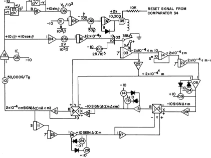
is in the first quaarant. This relation can be mechanized by a single amplifier and one multiplier (see ampli-fier 18, figure 5-1). This circuit makes use of the possibility of separating the TR-48 quarter-square multiplier into two independent X2 generators. The iteration scheme used is proportional correction:where an and E"n are the values of a and E" forthe nth rW1,
= E"- a
n n-1
The use of the plus or minus sign is determined by the following rule: The signs of .6an and .6E" n are compared; if they are alike, this is taken as an in-dication that da/d€ is positive, and the - sign is used. If they are W1like, the + sign is used.
Figure 5-1 gives the appropriate circuit. Ampli-fiers 06, 07, and 10 solve the dynamiC equations. The value of x is to be sampled when y crosses zero. This will not happen at the end of an operate cycle, but at some time during the cycle. Hence a comparator-controlled track- store W1it is used. When y crosses zero, comparator 35 flips to the minus side, switching amp 03 from TRACK to STORE. Amplifier 07 continues to integrate down-ward (this means a negative value of y, which has no physical significance). A feedback diode is used to prevent the output of amp 07 from becoming more negative than about half a volt. This is to prevent overload in case the OPERATE cycle con-tinues for a long time beyond the collision point (the length of the OPERATE cycle is fixed).
[image:15.615.338.563.34.131.2]Amplifiers 14 and 22 delay the stored error by one cycle (see Table 3-1 and Figure 3-2). Amplifier 14 (marked S*) behaves like an ordinary S (Storage) amplifier, but its mode control is a bit different from that described in section 3a. It cycles be-tween OPERATE and HOW instead of OPERATE and RESET. An ordinary Storage amplifier, as de-scribed in section 3a, could have been used, but this trick enables the amplifier to share a dual integrator network with amplifier 15, reducing the number of integrator networks required.
Amplifier 08 is a high-gain amplifier. Instead of a feedback resistor, it has a feedback limiter circuit designed to limit it to approximately :1:10 volts. The output of amp 08 may be thought of as essentially a digital signal, having the value -10 when E"
r?
E"n-1 and + 10 when E" n < E" n+ 1, or in more concise terms, its output is -10 sign (6 E" n)' Similarly, the output of amplifier 16 is + 10 sign ll.Ot. n, which has been computed from the value of 6Ot. for the last run, delayed one cycle. The signs of ll.Ot.n and ll.E"n are compared by multiplier 13, which acts as a "coincidence gate" or "exclusive OR" circuit. The output of amplifier 13 is -10 volts if 6Ot.n and6 E" n have the same sign, and + 10 volts if they have opposite signs. Multiplier 21 multiplies this logic signal by E" n, so that the output of amplifier 21 is proportional to :I: E"n, the sign depending on
the relative signs of 6Ot. n and 6E" n' The signs on the multipliers are chosen so that the output is proportional to -6Ot.~+ l' This signal is delayed by amplifiers 11 and 23 and converted to a binary signal by amplifier 16, so that it can be used to determine the direction of change for the next run.
The output of amplifier 21 is just what is needed for the iteration scheme 6 Ot.n+ 1 = :l:GE" n = -GE" n SIGN (Mn 6 E"n)' Pot 10 introduces the constant G and the appropriate scale factor. Its output is -10 6Ot.n+ 1/TR. Amplifier 15, the parameter up-dating integrator, is connected so that it operates when the main problem is in RESET and holds when the main problem is in the OPERATE mode. It integrates the constant -10.6an+ 11TR for a con-stant interval TR (the RESET time) and its output changes by an amount + 10 OOn+ 1 in this time. Thus its output, + 10 Ot.
=
+ 10 cosa
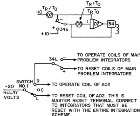
is appropriately up-dated during the RESET cycle and its new value is held during the following OPERATE cycle. Multi-plier 25 and amplifier 18, as described above, pro-vide the necessary squaring, subtraction, and square root functions to generate 10 sinO from the input 10 cos O.Figure 5-2 gives the circuit for the mode control cycling. The operation of this circuit was analyzed in detail in section 3-d. Note that the MASTER
TO OPERATE COILS OF MAIN 34L O=--PROBLEM INTEGRATORS
C::
TO RESET COILS OF MAINPROBLEM INTEGRATORS
SWITCH .R TO OPERATE COIL OF A02
-20 NO.1
~.oc
[image:16.620.316.560.55.257.2]VOLTS
~ TO RESET COIL OF A02. THIS IS MASTER RESET TERMINAL. CONNECT TO INTEGRATORS THAT MUST BE RESET WITH THE ENTIRE INTEGRATION SCHEME.Figure 5-2. Mode Control Circuitry for Boundary-Value Problem
RESET terminal. on switch #1 may be patched to the RESET, coil of the parameter-updating inte-grator 15, to enable a first-run value Ot.1 to be established on the integrator. The computer mode busses are completely unused, and all mode con-trol signals are obtained from the manual switch and the comparator. The -20 volt relay power supply is terminated on the TR-48 patch panel in a terminal marked RV (relay voltage). This terminal is in the lower left corner of the readout panel.
Since the RESET and OPERATE busses are not used in this circuit, the operation of the circuit will be independent of the mode pushbuttons on the control panel, except for the POT-SET mode, which closes a relay around every amplifier. The POT-SET mode is therefore a convenient one for setting all storage. amplifiers to zero before the start of the iteration. The sequence of operations to be performed by the operator is as follows:
1) Put the computer in the POT-SET mode to clear all storage to zero.
2) Put SWITCH #1 to left pOSition.
3) Depress the HOW pushbutton to bring the computer out of the POT-SET mode.
4) Put SWITCH #1 to the right position.
Results for a typical series of runs are given in figure 5-3. The target was placed at 2,000 feet, and a first-run value of a was chosen that gives an extremely large initial overshoot. Note that the results of successive runs approach the target mon-otonically, and that the amount of the correction decreases as the larget is approached.
Table 5-1. Potentiometer Settings
Pot Parameter Numerical
Number Description Setting
00 2R/105 0.040
01 g/103/{3 0.161
02 1/50{3 0.100
03 Vo}03 0.750
04 Limiter 0.470
05 a1 0.100
06 2Vo
f-°
5{3 0.07507 TR/Top 0.500
08 (TR + T >/TRT op op 0.300
09 Limiter 0.470
10 50,OOOG/TR 0.040
14 Limiter 0.470
19 Limiter 0.470
24 Limiter 0.470
29 Limiter 0.470
9,000
8,000
t1~
~I---It is worthwhile to pay some attention to the mean-ing of the constant G. The entire iteration scheme may be thought of as a feedback control system con-trolling the parameter O!. The correction is pro-portional to the error (, and the constant G may be thought of as the gain of the iteration scheme.
It is interesting to run the iteration scheme several times and observe the effect of the gain G on the convergence. As expected, low gain leads to slow convergence. Increasing the gain speeds the con-vergence, up to a point, but excessive gain produces divergence.
Table 5-2. Summary of Integrator Mode Patching
02, 03
06, 07 10, 11
14, 15
21, 23
From SWITCH 1.
From lower contacts on comparator 34 RESET coils from + terminal
OPERATE coils from - terminal
RESET coil patched to SWITCH 1, left terminal.
OPERATE coil from + terminal, com-parator 35
From lower contacts on comparator 34
RESET coils from - terminal.
OPERATE coils from + terminal. (The mode of these integrators is com-plementary to the mode of the main problem integrators)
COMPUTER RESULTS FOR 6 ITERATIONS OF BOUNDARY-VALUE PROBLEM, USING PRO-PORTIONAL CORRECTION. TARGET PLACED
7,000
rt'
7
\/
2,000 FEET FROM LAUNCHING SITE.'I
1\
V
~IIIUMBERS PERATE CYCLES. ON 'CURVES REF'ER TO SUCCESSIVE 6,000-
I-III5,000 III II..
>-4,000
3,000
2,000
1,000
0 0
'I
II
\ J
V\
1'\
X
\
\2
\
I
./ 4h
1\
\
fl
/
\
\
I /
54\
\
~,
..
\
\
T A r "
\
\
1,000 2,000 3,000 4,000 5,000 6,000 7,000 8,000 9,000 10,000 11,000 12,000 13,000 14,000 X (FEET)
[image:17.613.58.537.181.725.2]APPENDIX 1
PARAMETER SWEEP CIRCUIT
The NORMAL/SPECIAL option on the TR-48 inte-grator enables us to construct a very simple cir-cuit for the parameter sweepprobleminSection3a.
In Figure A2-1, integrator #1 is a SPECIAL inte-grator, while all the others, including the T and S (track .and store) integrators are operating in rep-op.
-10
I
50
TO ARM OF X-Y PLOTTER
SYSTEM OF DIFFERENTIAL X(t)
>'--...
-1 EQUATIONS (REP.-OP.)T
Figure A2-1
TO PEN OF X-Y PLOTTER
After every rep-op cycle, the S-amplifier stores the final value of the variable X. This final value will change gradually as ~ changes. Since '" is changing very slowly (it takes 50 seconds to go from zero to + 10 volts) it will appear very nearly constant from the point of view of the rep-op cir-cuit. In particular, if the rep-op rate is 20 .solu-tions per second, '" will Change by only 0.1 volt during a single computation. This is the smallest change that can be detected on the TR-48.
Thus, the rep-op circuit will solve the differential equations of the system for a virtually constant value of "', and the S-amplifier will store the final value X. After the next solution, the slightly dif-ferent value of '" will cause a small change in the value of X, and the output of the S-amplifier will change accordingly. With the <x.,. integrator con-nected to the arm and the S-amplifier concon-nected to the pen, the X- Y plotter will produce a graph of the final value X versus the parameter "'.
The graph should look something like Figure A2-2; that is, the graph will not be smooth, but will con-sist of many small steps. However, if <X varies
over the desired range in 50 seconds, and the rep-op rate is 20 solutions per second, the graph should consist of 1,000 steps, and they should be so small as to be barely noticeable.
X FINAL
-;---a
[image:18.617.54.296.210.345.2]APPENDIX 2
TR-48 RELAY MODE CONTROL
The mode control on the RMC TR-48 is accom-plished with relays which are energized from a
-20 volt DC power supply. The individual relay coils appear on the patch panel, which allows for independent control of integrator mode.
The relays normally receive inputs from two mode control busses, called the RESET bus and OP-ERATE bus. Each bus is energized from the corre-sponding pushbutton on the mode control panel:
1) When the RESET mode is selected with a pushbutton, the RESET bus is energized with -20 volts and the OPERATE bus is de-energized.
2) When the OPERATE mode is selected, the OPERATE bus is energized, and the RE-set bus de-energized.
3) ill the REP-OP mode, the RESET and OPERATE busses are energized alter-nately, thus cycling the computer between RESET and OPERATE.
4) When the HOW mode is selected, both busses are de-energized.
Each dual integrator network has two input termi-nals on the patch panel which go to relay coils. These terminals will be referred to as the RESET coil and the OPERATE coil. (This is an over Simplification - actually, one of the terminals energizes two relay coils, but this is not important from a programmer's point of view):
1) When the RESET coil is energized, the integrator is in the RESET mode.
2) When the OPERATE coil is energized, the integrator is in the OPERATE mode.
3) When neither coil is energized, the inte-grator is in HOW.
4) If both coils are energized Simultaneously, the integrator may be . in any of several modes. Because of this uncertainty, the programmer should avoid simultaneously energizing both coils.
ill normal operation, each coil is patched to the corresponding bus. The mode of the integrator
is then selected by the pushbuttons in the normal manner. This standard mode control connection can be made with a double horizontal bottle plug.
If this plug is removed, the coils can be patched in many different ways. For example, reversing the connections (RESET coil to OPERATE bus and OPERATE coil to RESET bus) gives a tracking unit, as described in Section 3a. illtegrator coils may also be energized directly from the -20 volt relay power supply or through comparators or manual switches. The relay power supply appears on the patch panel in the lower left-hand terminal of the readout panel, at the terminal marked RV (relay volts).
For some applications, it is desirable to have some integrators running in Rep-op and some in real time simultaneously. This result can be achieved on the TR-48 as follows: a shaded por-tion of the integrator network contains two holes marked NORMAL and two holes marked SPECIAL.
When the holes marked SPECIAL are patched together, the integrator operates normally. (When a bottle plug is used for this connection, the word SPECIAL is covered up. Hence the operator sees the word NORMAL when the integrator is operat-ing normally). When the holes marked NORMAL are covered with a bottle plug and the word SPECIAL is exposed, the integrator operates in a special manner, i.e., it goes into the OPERATE mode as soon as the REP-OP mode button is de-pressed, and remains in OPERATE (with a real-time capacitor, not a rep-op capacitor) as long as the computer is in repetitive operation. An applica-tion of such an integrator is given in Appendix 1.
One other feature of the TR-48 integrator network has been used in this article. This is the possibility of changing the feedback capacitor on an integrator to increase its integration rate. This feature allows a wider range of time-scale factors than would otherwise be the case. A bottle plug, called the (3 plug, is normally patched into each integrator. Removing this plug replaces the feedback capacitor by a capacitor of 1/10 the value, increasing the integration rate by a factor of 10. This feature operates independently of mode control patching, rep-op, NORMAL/SPECIAL connections or any-thing else. Whatever feedback capacitor the inte-grator would have with the (3 plug (a rep-op or "real-time" capacitor) is replaced by a capacitor of 1/10 the value. In contrast to the mode control connections, the dual integrator has two separate
@ plugs - one for each integrator in the network.
Note: The TR-48 with Electronic Mode Control (EMC) differs only slightly from the RMC Computer in so for as the programmer is
con-cerned, despite its completely different system of controlling the modes of integrators. The electronic switches, which replace the mode-control relays, are operated from logic signals, i.e., on the TR-48, a logical 1 = +5V and a logical 0 = OV. Hence, the busses which feed the mode switches operate at these two levels iust as
the RMC busses operate at -20V and OV levels. The following table illustrates EMC operation.
INPUTS RESULTING
IC OP MODE
1 0 RESET
0 1 OPERATE
0 0 HOLD
1 1 NOT ALLOWED
These inputs can be obtained by depressing the proper mode control buttons if the mode-control bottle plugs are patched, or by patching from devices which produce these levels (electronic comparators, gates, flip-flops, etc.). There is a terminal in the readout panel labeled +5V which can be used as alogical 1 level "supply". All other components on TR-48 dual integrator networKS apply to the EMC network as well as the RMC network.
In addition, EMC TR-48's are usually available with Electronic
Comparator moclu/es, which comprise one electronic comparator
net-work, two digitally-controlled analog switch networks, and two track-store amplifier networks. The latter obviate the need for using standard integrators as track-store devices and thus add to the flexibility of the computer. Electronic Comparator modules are also available for the RMC computer.
Symbols
1. Electronic Comparator (EC)
ANALOG
INPUTS e l - i " ' l . . . . - - I DIGITAL
e2----L-.../
Lo
OUTPUTSWhen el + e2 >0, the "I" output is at the "I" level When el + e2 < 0, the "I" output is at the "0" level 2. DIA Switch
INPUT OUTPUT
DIGITAL.
A N A L O G = Y ANALOG
COMMAND
3. TiS Amplifier
ANALOG INPUT
DIGITAL COMMAND
APPENDIX 3
TR-48/DES-30 HYBRID IMPLEMENTATION
0F
ONE PARAMETER OPTIMIZER (BOUNDARY VALUE) PROBLEM
The all-analog simulation of the trajectory prob-lem given in Section 2c is modified for hybrid implementation. The necessary logic functions are peiformed by the logic elements of the EAI DES
-30 Digital Expansion System
ANALOG PORTION
The analog portion of this problem is the part of figure 5-1 used to solve the equations 5-1 and 5-2.
It is repeated here for reference.
MODE CONTROL
The mode control program (see Figure A3-2) consists of DC A and FF C. Its purpose is to provide signals to alternately throw the TR-48 into
VO/IOOO
10SINe
- I O - - - - f
-10 +10
OP (9 seconds) and RS (9 seconds). The 9 sec period is dictated by the problem solution time -longer periods may be used if desired, but not shorter periods. The program also provides the signal necessary to control the OP-HD mode of integrator 15 - the one that operates O! = cos 9 from .6.O!n+ 1 during the time that the problem is in RS, and goes to HD when the problem is in OP. See the timing diagram in Figure 3A-3.
The LP permits manual start-stop. When the LP is pushed, DC A counts down at the rate of 1 count per second, producing a Co blip and reloading itself to 9. The Co blip triggers FF C so that its output is high for 9 seconds and low for another 9
seconds. Thus, the complementary outputs of FF C are just the signals necessary to control the OP, RS mode inputs.
>-.... __
.TO E.C.A.TO
Tis
Aa ) -_ _ _ _ _ .... -..;:I::!.::;..a n+ I, FROM D/A AMP. B FROM
RST _ _ _ ....
OM
DES-30 FROM
DES-30
[image:21.621.115.510.345.713.2]+ Y _ - r - - . , . .
RS OUT
(FROM A07) I - -...
+---+---{
TO -/j.Q n+1
INTEG.--...
<
15TO Ie OF INT. 15
Figure A3-2: Mode Control and Optimization Logic
OPTIMIZATION LOGIC
TIS A tracks the error, En, during the OP mode, while the altitude y is still positive (above ground). When y goes negative (the projectile hits the ground), comparator A goes low, and TIS unit A holds.
After the OP period is finished, the RS mode output throws TIS B into TRACK. It then tracks the output of TIS A (with sign inversion). Thus, on the next OP cycle, TIS A tracks the present error, En, while TIS B holds the old value, En-I. See timing diagram in Figure 3A-3.
OP-RS TIMING
-£n
(T/SA)
£n-I
(T/S B)
SAMPLE SGN ll£
SAMPLE SGN llan
INTEG 15
~
RSTRA~
STORE
TRACK
I
STORE
--.J
~
OPPEN CTL
Comparator B goes high whenever En-I - En > 0 (that is, when b. E is positive) and remains low when A.E is negative. Thus, its output may properly be called "sgn /),E". Flip flop B stores this information as of the instant when 1/S A goes to STORE -that is, at the earliest instant both.T/S A and TIS
Bare storing. This is achieved by disabling this Figure3A-.3:
MODE CONTROL
C
9SEC:=:/
r-L
[image:22.620.60.541.49.456.2] [image:22.620.315.562.474.719.2]
FF when T/S A goes to STORE. The same effect can be achieved by enabling FF B by a blip ob-tained from differentiating the trailing edge of Compo A output, but this would require a differen-tiator.
Note that FF B "tracks" sgn D. E throughout the time when y> O. It might be asked whether this has any adverse effect. It can be seen that this is not the case because integrator 15 is in HD through-out the period y> 0, so that it doesn't care abthrough-out sgn A E (or anything else, for that matter).
FF A is enabled by a blip which is the AND of Co and FF C - that is, a blip occurring just prior to going into the OP mode. At this time, the output of amplifier B has D.an on it, comparator C output is sgn b
an,
and so FF A stores sgn D.OU. Recall thatDan
is the quantity used to generate the parameter of interest, a n+ 1, that is, AO'n is determined during the OP mode of the previous run, not the one we are just going into.The outputs of flip flops A and B are compared in a negated XOR (Exclusive-Or) program. An XOR is basically a digital comparator - its output is high whenever the two inputs are unequal (one is low while the other is high). Thus the negated XOR output is high whenever the inputs are equal -both high or -both low. That is, the signal 6 in Figure 3A-2 is high whenever sgn D.En and sgn.6an are equal; in Boolean notation 0 = (sgn AE n).
(sgn D.an) + (sgn AEn) (sgn Aan); in algebraic notation 6 = (sgnAEn) . (sgnAan). Thus, the XOR
programs replaces multiplier 13 in the all-analog implementation of this program.
Amplifier B and the associated electronic switches control the selection of the sign in the equation AOfi+ 1 = ± GE in accordance with the signal 5 just described:nwhen 6 = 1, indicating that sgn AEn and sgn D.an are equaI, the output of amplifier B is + En; when 6 = 0, -E n. (Recall that integrator 15 requires - D.0fi+ 1 at its input). Thus, amplifier B and its switches replaces multiplier 21 in the all-analog simulation.
INITIALIZATION
In all programs of this type, initialization should carefully be considered. Initialization consists of two problems: 1) How does one get the problem started? (This is no more a simple analog set-up; we also have a digital section to worry about, and simply pushing the OP button on the TR-48
won't do!) 2) How does one make sure that all initial conditions are proper, both analog and digital?
The question of starting (and, inCidentally, the related question of stopping) has been taken care of by the LP in the mode control section. When the LP is released, FF C is cleared, and the TR-48 is in RS. This assumes that the clock is running and the TR-48 is in SLAVE - which is the normal state of affairs in hybrid simulations when running. When the LP is latched, DDC A starts counting and· the simulation is under way.
The question of digital il~itial conditions is that of the correct initial states of flip flops (GPR FF, DC FF, MT & DIF FF, etc.) For example, we may wish to set DC A to 09 manually so the cycle starts in the RS mode. If DC A is cleared, the cycle starts with OP mode. But most importantly, we must decide whether FF's A and B should be cleared or set to begin with. If we know what sgn
/'I.oc nand sgn /'I.E n are for the first two run (and in this problem we can find this out because it hap-pens to be a very Simple one), then we can set FF's A and B accordingly. If we do not know, as will be the case in a more sophisticated problem, then we must program an initialization run to determine the initial quantities. In this particularly simple situation, we can ignore the initial setting of FF's A and B altogether. This results in at most 2 bad runs (the first two) in which the optimization may go in the "wrong direction". However, after T/S A and T/S B have had a chance to operate once, things will quiet down.
A LIST OF MNEMONICS (DES-30)
C Carry Out
0
DC Down Counter
DIF Differentiator
EMC Electronic Mode Control
FF Flip Flop
GPR General Purpose Register
HD Hold Mode
LP Latching Pushbutton
MP Momentary Pushbutton
MT Monostable Timer
OP Operate Mode
RS Reset Mode (IC)