Compact microscope system
for biomedical applications
Thesis by
Jinho Kim
In Partial Fulfillment of the Requirements for the degree of
Doctor of Philosophy
CALIFORNIA INSTITUTE OF TECHNOLOGY Pasadena, California
2017
2017
ACKNOWLEDGEMENTS
All of achievements I made at Caltech would not be possible without the help of others I have worked with. First of all, I would like to express sincere appreciation to Professor Changhuei Yang about his thoughtful guidance on the research. His advice always led me to consider problems from different perspectives and helped me to find solutions eventually. I also want to thank him for giving me enough chance to design and organize optical systems by myself. I have learned a lot about the system level design during the process, and I actually enjoyed the whole process of engineering work.
I was lucky enough to work with brilliant collaborators from in and outside of Caltech in every project. Professor Ana Rodriguez from New York University taught me about parasitology and biological sample treatment in ePetri project. I had asked her a lot of different types of sample preparation and she was always willing to helping me on my request. Professor Henry A. Lester, Dr. Beverley M. Henley, and Charlene H. Kim helped me to prepare primary mouse ventral midbrain neurons for the EmSight project. I have learned a lot about neuro-biology and in vitro cell culture work from them. Dr. Han Xu and
Dr. Dana Nojima from Amgen helped me to bring out the idea of high throughput parallel imaging system, and they also gave me lots of practical ideas about the 96Eyes project. I really appreciate all of the inputs from the collaborators.
Caltech Biophotonics lab has provided me the best working environment I can ever imagine. I was really happy to work with smart and friendly lab members at the Biophotonics lab. I would like thank them for their help: Seung Ah Lee, Jaehee Jung, Chao Han, Jiantao Huangfu, Daifa Wang, Roarke Horstmeyer, Xiaoze Ou, Mooseok Jang, Shin Usuki, Donghun Ryu, Hao Deng, Yidong Tan, Edward Zhou, Haowen Ruan, Atsushi Shibukawa, Albert Chung, Josh Brake, Michelle Cua, Helen Lu, and Jian Xu. And I want to express special appreciation to Antony Chan and Daniel Martin who are upgrading the imaging system I have built here in Caltech. And our lab manager, Ms. Anne Sullivan, has been my best supporter during my stay at Caltech. I appreciate all of the assistance she has given to me so far.
ABSTRACT
Demands for an imaging system which has high space-bandwidth product (SBP) are increasing in modern biomedical research as the amount of information to be dealt with is increasing. However, conventional microscopy has a limited SBP of about 10 mega pixels, and as such if a user wants an image in high resolution, the field of view (FOV) of the image is reduced, or if a wide FOV is necessary, the user needs to give up the resolution of image. A common way of overcoming this SBP limit in the conventional microscopy is to use mechanical moving stages and scan through wide sample area, however, it is time consuming to image large area using a high numerical aperture (NA) objective lens. This thesis presents compact imaging systems based on Fourier ptychographic microscopy for biomedical applications which are able to increase SBP without having any mechanical moving parts: one imaging system for an incubator embedded imaging system to be used in in-vitro cell
Acknowledgements………...iii
Abstract ………v
Table of Contents………. vi
List of Illustrations ... viii
List of Tables ... ………x
Chapter 1: Introduction to optical microscope systems ... 11
1.1 Principle of optical image formation ... 11
1.2 Modern microscopy systems ... 14
1.2.1 Kohler illumination ... 15
1.2.2 Photo detectors ... 17
1.2.3 Objective lens ... 19
1.2.3.1 Resolution ... 20
1.2.3.2 Field of View ... 22
1.2.3.3 Depth of Field ... 23
1.3 Aberration ... 23
1.3.1 Chromatic aberration ... 23
1.3.2 Achromatic aberration ... 25
1.3.2.1 Tilt ... 25
1.3.2.2 Defocus ... 25
1.3.2.3 Astigmatism ... 25
1.3.2.4 Coma ... 27
1.3.2.5 Spherical aberration ... 27
1.3.2.6 Strehl ratio ... 27
1.4 Imaging modes ... 27
1.4.1 Bright field intensity imaging ... 27
1.4.2 Zernike phase contrast imaging ... 29
1.4.3 Differential interference contrast imaging ... 30
1.4.4 Fluorescence imaging ... 31
Chapter 2: Fourier ptychographic microscopy ... 33
2.1 FPM image acquisition process ... 33
2.2 FPM image reconstruction process ... 38
2.3 Image space-bandwidth product improvement ... 42
2.4 Digital image refocusing ... 43
2.5 Computational aberration correction ... 44
Chapter 3: EmSight: Incubator embedded cell culture imaging system ... 46
3.1 Introduction ... 46
3.2 System configuration ... 48
3.3 LED matrix and EmSight positional calibration ... 51
3.4 System characterization ... 54
3.6 Dual channel fluorescence imaging ... 67
3.7 Discussion and conclusion ... 71
Chapter 4: 96Eyes: High throughput 96 well plate imaging system for fast drug screening ... 73
4.1 Introduction ... 73
4.2 System configuration ... 76
4.2.1 Imaging sensor board ... 77
4.2.2 Injection molding polymer objective lens ... 80
4.2.3 LED matrix operation for FPM illumination ... 81
4.3 System characterization ... 85
4.3.1 Image resolution of 96Eyes ... 86
4.3.2 Digital image refocusing of 96Eyes ... 91
4.3.3 Fluorescence imaging of 96Eyes ... 94
4.3.4 Comparison between 96Eyes and commercial well plate imaging systems ... 99
4.4 Discussion and conclusion ... 99
Number Page
1.1Optical imaging system diagram ... 12
1.2 Finite corrected and infinity corrected imaging system ... 13
1.3 Configuration of modern optical microscope ... 15
1.4 Microscope illumination path. Kohler illumination ... 16
1.5 Microscope imaging path ... 17
1.6 Microscope Objective lens ... 18
1.7 Systems with annular pupil ... 21
1.8 Chromatic aberration ... 24
1.9 Bright field imaging modes ... 28
1.10 Fluorescence imaging ... 31
2.1 FPM image acquisition process ... 34
2.2 FPM illumination methods ... 36
2.3 Phase retrieval algorithm ... 38
2.4 FPM image reconstruction process ... 40
2.5 FPM image resolution improvement ... 42
2.6 FPM digital image refocusing ... 43
3.1 System configuration and imaging method of the EmSight ... 49
3.2 LED position calibration ... 52
3.3 Effect of LED position misalignment ... 53
3.4 Raw image resolution of EmSight ... 54
3.5 FPM reconstructed image resolution of EmSight ... 55
3.6 Multi-modal imaging of EmSight ... 56
3.7 Digital refocusing of the EmSight ... 57
3.8 Digital image refocusing example ... 60
3.9 Large FOV imaging of the EmSight ... 61
3.11 6-well plate imaging of the mouse ventral midbrain culture ... 64
3.12 Time-lapse imaging of the dividing cells ... 67
3.13 EmSight with dual channel fluorescence imaging ... 68
3.14 FPM imaging of dual channel fluorescence EmSight ... 69
3.15 Dual channel fluorescence imaging of dual channel fluorescence EmSight ... 70
4.1 96Eyes system configuration ... 74
4.2 Imaging sensor board operation ... 75
4.3 Cooling of imaging sensor system ... 78
4.4 Injection molding polymer objective lens ... 79
4.5 CODE V ray tracing simulation result ... 81
4.6 LED matrix operation for FPM illumination ... 82
4.7 FPM image acquisition process ... 83
4.8 FPM resolution test of 96Eyes ... 84
4.9 FPM intensity imaging test of 96Eyes ... 85
4.10 FPM phase imaging test of 96Eyes ... 87
4.11 96 well plate bottom height distribution ... 88
4.12 Digital refocusing of 96Eyes ... 89
4.13 Digital refocusing of HeLa sample in 96 well plate ... 93
4.14 96Eyes fluorescence imaging ... 94
4.15 96Eyes fluorescence imaging test using 2 µm fluorescence beads ... 95
4.16 96Eyse fluorescence imaging test using GFP HeLa cell lines. ... 96
4.17 Bright field image comparison between 96Eyes and Operetta ... 97
Number Page
1.1Microscope tube length and objective thread size Mercury ... 19
1.2PSF and resolution of systems with rectangular and hexagonal pupil 22 1.3Zernike aberrations ... 26
1.4Wavelength for maximum absorption and emission ... 32
4.1 Dispersion of the materials used in the objective lens ... 80
4.2 Fluorescence imaging throughput comparison ... 101
C h a p t e r 1
INTRODUCTION TO OPTICAL MICROSCOPE SYSTEMS
An optical microscope is a fundamental instrument for inspection and examination of minuscule samples in biological and medical research. The main reason that the optical microscope has gained such popularity in a wide range of applications is that it is able to convert small, closely located samples, which are not discernable to our naked eyes, into clearly separated entities in large detectable sizes without ambiguity. Since its first invention in the 17th century, there have been several different approaches for better magnification and resolving power. However, their working principles share a common background in the sense that they are utilizing light as a medium for sample information transfer.
As an introduction to this thesis, we will explain the basic working principle of the modern optical microscope in this chapter. The ray properties of light in image formation and the configuration of modern microscopes are briefly described. Following this, several different modes of optical microscopy are introduced at the end of the chapter.
1.1 Principle of optical image formation
approximate image of the sample information, and a user gauges the actual sample information based on the measured image information and the specifications of the imaging system in use.
Light travels in an imaging system by obeying Fermat’s principle [1]:
Light rays travel along the path of least time.
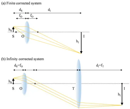
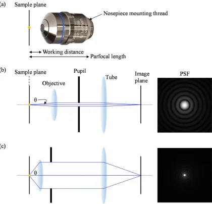
Because light has a different speed when it travels in different materials (by the ratio of refractive index), the light ray changes its direction by Fermat’s principle when it encounters a new material. The lens is an optical part which utilizes this property of ray propagation to focus light rays that are parallel to the optical axis into a point, after traveling a designed focal length. Any lens component shown in this thesis can be described as a singlet lens or can be composed of multiple lens elements inside. In the case of a lens with multiple elements, we can replace the position and the focal length of a single lens with the principal plane and the effective focal length of a multi-element lens, respectively. In a finite corrected imaging system, a single objective lens, which is designed to correct optical aberrations at a fixed tube length, is used for image formation, as shown in Figure 1.2(a). By similarity of triangles in rays, the size of a sample (S) is magnified (or demagnified) by Equation (1.1):
M ≡ . (1.1)
Figure 1.1: Optical imaging system diagram
Sample
Light
This type of configuration has an advantage in system complexity because only one lens is required in order to generate an image of the sample. However, it has a limited degree of freedom in the sample location for the best image formation, because the sample position (dS) and objective focal length (fO) are also coupled with the image’s position (dI) by the
Gaussian Lens formula [2]:
[image:13.612.112.541.88.448.2].
(1.2)Figure 1.2: Finite corrected and infinity corrected imaging system. S: sample, O: objective lens, T: tube lens, I: image, dS: sample distance, dI: image distance, fO: objective focal
we can only get the designed magnification of the image from just one possible position of sample. Furthermore, every optical component in the imaging system needs to be considered when designing the objective lens, because any additional parts in the imaging system between the objective lens and imaging plane would affect the system’s aberration correction.
Infinity corrected imaging systems are another type of imaging system (Figure 1.2 (b)). Aberration of the infinity corrected objective lens is best corrected when the sample is located at the focal plane of the objective. As a result, light rays become parallel after passing through the objective lens, which makes an image of the sample positioned at infinity from the lens. An additional lens (tube lens) is used in the system in order to focus the image location to a closer distance. One of the advantages of an infinity corrected system is that the distance between the objective lens and the tube lens is flexible. In Figure 1.2 (b), the distance between the two lenses is set as the summation of the focal lengths of each, in a configuration known as the 4f imaging system. However, the separation between the lenses can be any distance as long as any rays passing through the objective lens can be collected by tube lens without loss. Along with the freedom of choosing the distance between the two lenses, this imaging system allows the user to modify it with less aberrations than the finite corrected system when inserting extra optical parts between the objective and the tube lens because all the rays are parallel in this region. Unlike finite corrected systems, the magnification of an infinity corrected system is only determined by the optical properties of the lenses in use, which is easily derived from the Figure 1.2(b) using the similarity of triangles in rays:
M ≡ . (1.3)
1.2 Modern microscopy systems
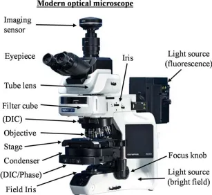
plane of the tube lens. The sample is usually loaded on the X-Y stage and the focus knob moves the sample stage or the objective lens nosepiece in order to focus the sample. There are two light sources installed in the microscope for sample illumination. One light source is used for transmission bright field imaging, and a more powerful light source is usually used for epi-fluorescence excitation. Additional filter cubes, phase rings, prisms, and polarizers are used for the specific imaging modes, such as fluorescence imaging, Zernike phase contrast imaging, and differential interference contrast (DIC) imaging.
1.2.1 Kohler illumination
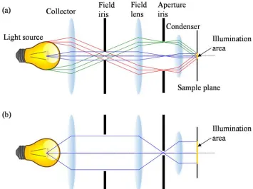
[image:15.612.170.477.93.375.2]gives us easy control of the illumination. By positioning one iris (field iris) on the sample conjugate plane and the other iris (aperture iris) on the source conjugate plane, we can control the size of illumination and the angle of illumination independently of each other. Two opposite types of illumination methods are shown in Figure 1.4 as examples. A field iris determines the size of illumination, and an aperture iris determines how many source points contribute to the illumination on the sample and controls the maximum angle of illumination as a result. When the field iris is small and the aperture iris is large (Figure 1.4(a)), the illumination area on the sample plane is small but the illumination is made from multiple angled illumination sources, thus generating an incoherent illumination scheme. On the contrary, when the field iris is large and the aperture iris is small (Figure 1.4(b)), the light source illuminates a large area on the sample plane. However, the small aperture blocks light from most of the source points and passes light only from a small point source which generates a spatially coherent direct planar illumination.
1.2.2 Photo detectors
[image:17.612.132.525.84.356.2]electrons directly at the position of the photodiode and transfer the voltage as an output. However, CCD imaging sensors transfer the generated electrons as an output and amplify them at the final stage of the sensor. Due to this difference, CMOS sensors have relatively small pixel sizes and a fast readout speed, however, they will usually have more noise related with voltage readout. On the contrary, CCD sensors have less noise, but have relatively large pixel sizes and slower speeds.
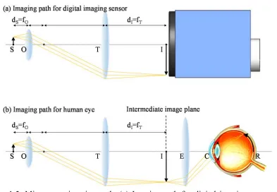
For the direct inspection of the generated image, we can direct the imaging path to our eyes. Unlike the digital imaging sensor, the human eye has its own light refracting parts (such as the cornea, aqueous humor, and lens), so an additional lens (eyepiece) is necessary in order to relay the image from the intermediate image plane to a plane which the human eye can focus into an image in its most relaxed state (usually 25 cm from the eye). Because our eyes demagnify the image by about 10 times when the sample is about 25 cm away (following Equation (1.1)), eyepieces usually have a 10X magnification in order to compensate this. 1.2.3 Objective lens
The objective lens is one of the most critical parts in a microscope system, which affects the quality of the image in many aspects. In order to give information on the objective’s design specifications, the magnification of the objective, the numerical aperture (NA), the aberration correction type, the field number (FN), and the amount of coverglass thickness correction are usually listed on the label of the objective lens. Because most objective lenses are composed of several lens elements for aberration correction, it is not easy to focus the sample using the effective focal length of the objective lens. For the practical usage of the objective lens, many lens makers provide additional information such as the working distance and parfocal length as shown in Figure 1.6 (a). Because objective lenses from each lens maker are designed to be working with the microscope frame produced by the same companies, careful attention is required when using objective lenses with a microscope frame of different company. First, due to the difference in tube length, the magnification of the
Table 1.1: Microscope tube length and objective thread size.
Company
Tube length
[mm]
Thread size
Leica
200
M25
Nikon
200
M25 / M34
Olympus
180
RMS
Additionally, the aberration correction of some objective lenses are designed together with the tube lens, so the image quality could be affected when it is used with other tube lenses. In table 1.1, microscope tube lengths and objective lens thread sizes of commonly used microscopes are listed.
1.2.3.1 Resolution
There are several definitions about image resolution, and one of the most popular definition is the Rayleigh criterion of two point sources. As described by the Rayleigh criterion [3], two nearby point sources are resolved when the peak intensity of the second point source image is located at the first minimum intensity of the first point source image. In order to use the Rayleigh criterion for image resolution, we need to know the characteristics of the image generated by the imaging system from a point source. The point spread function (PSF) is the irradiation distribution in the image plane from a point source. Using Fraunhofer diffraction theory [3], the PSF for a circular pupil has the shape in Equation (1.4):
,
(1.4)where J1 is the first order Bessel function of the first kind, and ≡ / , where is
distance in polar coordinates, D is the diameter of the pupil, and is the wavelength of light. The first zero of the above intensity distribution occurs at r=1.22 as shown in Figure 1.7 (b), which leads to the famous Rayleigh resolution criterion as shown in Equation (1.5):
1.22
/≅ 0.61
,
(1.5)Because the shape of the pupil is directly related with the PSF and image resolution, there has been large effort on the engineering of pupil function. It is called “apodization” [3]. One of the basic approaches in apodization is to make a central light block on the pupil, making an annular pupil as shown in Figure 1.7 (a). The PSF for an annular pupil [4] has the form of Equation (1.6) and the intensity distribution of the PSF by variation of the obscuration ratio ϵ is shown in Figure 1.7 (b).
.
(1.6)There are two distinct changes in the PSF when the obscuration ratio ϵ increases. The first minimum intensity occurs at shorter distance from the peak intensity location, which reduces the smallest resolvable feature of the system. However, the intensity in the second maximum peak increases when ϵ increases, which generates ringing noises in the final image and reduces the quality of the imaging system. For the rectangular pupil and the hexagonal pupil, the PSF and resolution are listed in the Table 1.2 for reference [4].
Figure 1.7: Systems with annular pupil. (a) Diagram of annular pupil. (b) Intensity distribution of PSF in systems with circular and annular pupil.
0 0.1 0.2 0.3 0.4 0.5 0.6 0.7 0.8 0.9 1
0 0.5 1 1.5 2 2.5 3
I( r) r ϵ=0 ϵ=0.25 ϵ=0.5 ϵ=0.75 Circular pupil
(b) Intensity distribution (a) Annular pupil
1
Because the image is detected by photodetectors in the imaging system, the final system resolution is determined from both the diffraction limited optical resolution and the pixel size of the photo detector as in Equation (1.7):
max
,
2
. (1.7)
When the system resolution is determined by the size of the PSF central peak, the system is called “diffraction limited”. Otherwise, the system is called a “pixel limited” system.
1.2.3.2 Field of View
The field of view (FOV) of an imaging system is the area on the sample plane which a microscope can form an image simultaneously on the intermediate image plane. This is characterized by the field number (FN) of the objective lens which indicates the diameter of the imaging field on the intermediate image plane (back focal plane of the tube lens). As a result, it is desired to make the size of an imaging sensor on the intermediate image plane
Table 1.2: PSF and resolution of systems with rectangular and hexagonal pupil.
Pupil Diagram PSF Resolution
Rectangular
Hexagonal
x y
a ϵ·a
x y
larger than the FN of the objective lens. The system FOV is determined by comparing the size of the imaging sensor and the FN of the objective lens as in Equation (1.8):
System FOV
min
,
.
(1.8)1.2.3.3 Depth of Field
The depth of field (DOF) is the axial distance from the sample focal plane which simultaneously makes a focused image in the intermediate image plane. As a result, it is related with the axial resolution of an imaging system and is defined as in Equation (1.9) using the wave nature of light [3]:
DOF
∙.
(1.9)Because the DOF has inverse square relation with the NA, it becomes more difficult to focus a sample using a high NA objective lens. In other words, a low NA objective lens has poorer axial resolution and needs additional methods for 3D sectioning of the sample.
1.3 Aberration
All the above discussion on image formation using an optical imaging system is based on several approximations about wave and ray properties of light propagation. The actual position, size, and shape of the generated image are slightly different from the theory. The deviation of the actual image from the theoretical approximation is called “aberration” of the system [5, 6]. There are many different sources of aberration in an imaging system. Material property, design parameters, and fabrication tolerance of optical elements all affect the way light propagates and become common sources of aberration. Even in the perfectly fabricated optical elements as defined by theoretical design, the theory itself contains several approximations, such as the paraxial approximation and thin lens approximation. It is best if the imaging system corrects the inherent aberration using systematic design; however, it is impractical to design an optical system which corrects aberrations with regard to all possible imaging applications. As a result, it is important to know how much and what types of aberration exists in the imaging system and what is the source of the aberration.
Chromatic aberration arises due to the dispersive nature of light in the refractive optical elements when polychromatic light is in use [2]. Refractive index is a material property which determines how light rays refract when it encounters a new material by following Fermat’s principle. The main source of chromatic aberration is dependent on the differences in refractive index of the wavelengths that make up the polychromatic light. By the lens maker’s law [2] of Equation (1.10), the focal length of a lens changes by the wavelength of light, which results in chromatic aberration in the imaging system.
1
,
(1.10)where n(λ) is the refractive index which is a function of wavelength λ, and R1 and R2 are the
radius of curvature of the two sides of the lens. Because different colored lights have different focal lengths from the same lens, they make different images due to the chromatic aberration as shown in Figure 1.8. The effect of chromatic aberration on the image is twofold. The images from different colors have different image planes in the axial direction, and cannot be focused simultaneously when the DOF of the system is small. This is called the “axial chromatic aberration.” Not only is this the result of the aberration, but the images from different colors have different spatial magnification, which generates two different sized images with different colors. This is called the “lateral chromatic aberration”.
At least two different materials of different dispersive power are necessary in order to correct chromatic aberrations. The most common index for material dispersive power is the Abbe number as in Equation (1.11):
,
(1.11) where d, F, and C are the Fraunhofer lines for wavelengths 587.6 nm, 486.1 nm, and 656.3 nm, respectively. The lower the Abbe number, the greater the dispersive power. By how many Fraunhofer lines are corrected in chromatic aberration, the commercial objective lenses are designated as achromatic, semi-apochromatic, and apochromatic lenses in increasing order of corrective ability.1.3.2 Achromatic aberration
When a monochromatic light source is used in the imaging system, there exists other types of aberrations other than chromatic aberrations. For an imaging system which has a circular pupil, the possible aberrations of an imaging system that is rotationally symmetric about its optical axis have the shape of phase variation on the pupil function. There are several different expressions on the phase pupil function, and it is commonly expanded in terms of Zernike circle polynomials. Each Zernike orders are called Zernike aberrations. In Table 1.3, the first 15 terms of Zernike aberrations are listed along with their phase map and PSF.
1.3.2.1 Tilt
When there is any phase gradient on the pupil function into a certain direction, it is called tilt aberration. Because the tile aberration shifts the PSF function without modifying its shape, the final image also shifts the same ratio while maintaining the quality of the image.
1.3.2.2 Defocus
When the image is observed at a different plane rather than the actual image plane, or when one of the imaging elements of the system is displaced along its optical axis, defocus aberration arises. Because the center intensity of the PSF is darker than the surrounding intensity, it generates a blurry image rather than a focused image.
1.3.2.3 Astigmatism
intensity (energy) along both rays is weaker than in other directions, which result in the elongation of an image in certain directions symmetrically.
1.3.2.4 Coma
Coma aberration is created when the principal rays and marginal rays of an off-axis sample are not coincident at the image plane. As its name suggests, its PSF looks like a coma. Due to the asymmetry of the PSF, the image affected by coma aberration smears into a certain direction.
1.3.2.5 Spherical aberration
Spherical aberration is an aberration related with the shape of an optical element. If the curvature of an optical element is not parabolic, not all of parallel rays coincide at a focal point. Due to the strong secondary rings in the PSF, an image suffering from spherical aberration has ringing noises around the boundary.
1.3.2.6 Strehl ratio
As seen in Table 1.3, the energy in PSF from aberrated systems are not concentrated like that from aberration-free systems, but spread into nearby areas. As a result, the energy of sample would also be spread into nearby areas when an image is generated from the aberrated system, which would reduce the quality of the image. The Strehl ratio is a commonly used index for aberration status of an imaging system [6]. For a given total power in the pupil, the value of the central irradiance for an aberrated pupil relative to its value for an unaberrated pupil is called the Strehl ratio of the imaging system. When the Strehl ratio is larger than 0.8, the system is called “diffraction limited,” otherwise it is called “aberration limited.”
1.4 Imaging modes
Modern microscopes have multiple imaging modes which are suitable for specific applications. In this section, we describe the basic imaging principles of typical imaging modes.
The most fundamental imaging mode is the bright field intensity imaging as shown in Figure 1.9 (a). In conventional Kohler illumination, the sample is illuminated by incoherent multiple light sources, and as such, the intensity of the sample information is transferred into the image. When the sample, described by s a ∙ , where a and ϕ are real valued functions, is illuminated by incoherent light sources, the image is formed by Equation (1.12) following Fourier optics [7]:
i ∙
∙ | | ⨂ , (1.12) where and are the Fourier transform and inverse Fourier transform, respectively, OTF is the optical transfer function which has a Fourier transform relation with the PSF, and ⨂ is the convolution integral operator. In bright field imaging, the image is the result of the convolution integral of the sample intensity distribution and the point spread function of the imaging system.
1.4.2 Zernike phase contrast imaging
When the sample is transparent, such as most biological samples are, then the bright field intensity image does not give us much detail about the sample because it only uses intensity (light absorption) information of the sample it is imaging. For those transparent samples, imaging the phase of the sample gives much more useful information about the sample’s details. In 1935, Zernike invented a method to record the phase changes introduced by the sample using a photodetector, and it is called Zernike phase contrast, or just phase contrast, microscopy [3]. The basic working principle of Zernike phase contrast imaging is shown in Figure 1.9 (b). In phase contrast microscopy, an aperture ring is positioned at the location of the aperture iris of the condenser lens. Due to this aperture ring, only certain angles of illumination are made on the sample, which constitute zeroth order diffraction directions. Along with the aperture ring, a special objective lens also contains a phase plate inside at the back focal plane of the objective lens. The phase plate also has a ring shape and matches the size of the ring with the size of the aperture ring, making phase changes only to the zeroth order diffraction from the sample. Let’s assume the sample is perfectly transparent and only has phase changes like those described by . We can expand into a Fourier series,
∑
∙ , (1.13)where is the coefficient of the mth order diffraction, and d is the fundamental period of . Let’s assume that the phase variation of the sample is small, such that the magnitude of is small compared to unity. Then can be approximated as,
1
, ∗ ( 0). (1.15) In phase contrast imaging, the phase plate inside the objective lens makes a one-quarter phase delay only onto the zeroth order diffraction. As a result, the diffraction coefficients change after passing through the phase plate like Equation (1.16):, ( 0). (1.16)
The resultant image on the photo detector is described by Equation (1.17):
i
|
| ≅ 1 2
. (1.17)Unlike the image Equation (1.12) produced by bright field intensity imaging, the phase changes introduced by the sample are transformed into changes in intensity of the image, which are recorded using a general photodetector. Zernike phase contrast imaging is a useful mode in imaging transparent biological samples; however, if the sample is thick and phase variation is not small compared to unity, noise related with additional phase terms are added into the final image.
1.4.3 Differential interference contrast imaging
of the image in DIC imaging. Because DIC utilizes birefringence as its working principle, it is not compatible with birefringent samples.
1.4.4 Fluorescence imaging
Fluorescence imaging is another frequently used imaging modality in modern microscopy. Fluorescence imaging utilizes light-matter interaction in fluorescing molecules (fluorophores). By quantum mechanics, there are several energy states in which molecules can reside. When molecules in the ground electronic state (S0) are illuminated by a light source of frequency (ν), part of the photons in the light source are absorbed by the molecules and excite them into higher energy states. Because there exist vibrational states and rotational states near these electronic states, light from certain bands of the spectrum can be absorbed by fluorophores. Naturally, it is called the absorption spectrum of a fluorophore. Once a molecule is excited, it quickly loses energy by vibrational relaxation and goes to the closest electronic state (S1). Due to the statistical nature of electron distribution, the excited molecule emits a photon of frequency (ν′), and returns back to ground state (S0). Because this light emission process is spontaneous, there is no relation between the emitted lights and they are incoherent of each other. Due to the energy loss during vibrational relaxation, the frequency of the emitted photon is always lower than the frequency of the absorbed photon (ν ν′). This energy loss process is called “Stokes shift.” The Jablonski energy diagram of the fluorescence imaging process, as well as the absorption and emission spectra of green fluorescence protein (GFP), is shown in Figure 1.10. More detailed information on the Figure 1.10: Fluorescence imaging. (a) Fluorescence imaging principle. (b) Absorption and emission spectra for GFP.
0 0.1 0.2 0.3 0.4 0.5 0.6 0.7 0.8 0.9 1
300 350 400 450 500 550 600 650 700
Wavelength [nm]
Emission Absorption
Absorption Spontaneous emission
(a) (b)
Vibration relaxation
Stokes shift
absorption and emission spectrum, excitation/emission filter, and dichroic beam splitter of fluorophores can be found at [8]. In Table 1.4, wavelengths for maximum absorption and emission of commonly used fluorophores are listed for reference.
Table 1.4: Wavelength for maximum absorption and emission.
Fluorophore
Absorption
[nm]
Emission
[nm]
DAPI
359
491
Alexa 350
343
440
CFP
436
477
FITC
495
519
Alexa 488
499
520
GFP
489
511
TRITC
550
573
YFP
514
527
Texas Red
589
610
mCherry
587
610
C h a p t e r 2
FOURIER PTYCHOGRAPHIC MICROSCOPY
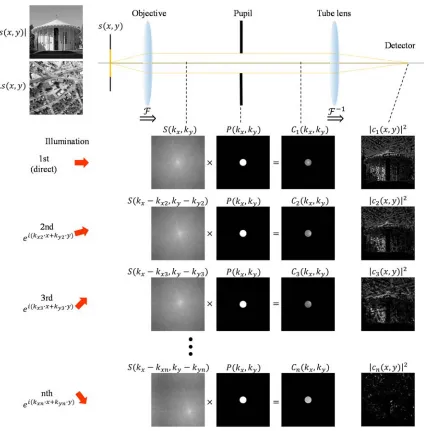
Fourier ptychographic microscopy (FPM) is a recently developed computational microscopy method which can improve the space-bandwidth product (SBP) of an imaging system by effectively increasing the resolution of a captured image using computational reconstruction algorithms [9]. FPM borrows ideas from conventional ptychography and the synthetic aperture. The word ptychography is a compound word of Greek words which means “to fold” and which means “to write.” As a whole, ptychography means a method of mathematically folding two functions together using convolution. Historically, it was first used by a German physicist Walter Hoppe to describe coherent diffractive imaging (CDI), a conventional ptychographic microscope [10]. Conventional ptychography captures multiple diffraction images from different parts of a sample using a coherent light source. Because each diffraction pattern is obtained from a region which overlaps with other parts of the sample, there is a large degree of redundancy in the captured data which is used to retrieve the phase information from the diffractive intensity measurements. On the other hand, Fourier ptychography captures multiple images from the same part of a sample using different illumination sources. Here, the overlap is made on the Fourier spectrum of the captured images. In this chapter, the working principle and imaging process of FPM will be explained.
2.1 FPM image acquisition process
captured by a photodetector (i x, y | , | ). This process is summarized in Equation (2.1).
i x, y , ∙ ,
, ∙ , . (2.1)
In an aberration-free imaging system, the pupil function P has a shape of top hat function in amplitude and does not have variation in phase. The pupil function of aberration-free imaging system can be described as Equation (2.2):
P , 1,
0, , (2.2) where kc is the cutoff spatial frequency of the pupil function which determines the maximum
allowed amount of information through the aperture and is defined as ≡ 2 . In the case of direct planar illumination, because the pupil function transfers only low spatial frequency terms from sample information, the captured image is basically a low pass spatially filtered version of the sample.
In Fourier ptychography, we make minor movements of the sample spatial spectrum S , and capture multiple images from different spectral locations of the sample. Because the movements are made in the spatial frequency domain of the captured images, the sample position of the illumination does not change, but the direction of coherent illumination on the sample changes. If we illuminate the sample from direction, the illumination wave adds an additional phase gradient through the direction on the sample plane as Equation (2.3):
∙ . (2.3)
If the sample is thin under the 1st Born approximation [11], the extra phase gradient directly applies into the sample field information and propagates through the imaging system together with the sample information as Equation (2.4):
illumination conditions, and they all have different spatial spectral information about the sample which will be used later during the image reconstruction process.
In order to make varying angled coherent light illuminations, a single light source can be modulated to change its light direction, or multiple light sources are used to illuminate the sample from different source positions. A simple method of changing the illumination angle from a single light source is shown in Figure 2.2 (a). In Kohler illumination, the angle of illumination is controlled by the aperture iris of a condenser lens. If we replace the aperture iris with a moving aperture stop or spatial light modulator (SLM), we can control the location of the passing light beam and modulate the angle of illumination. This type of illumination method can be easily adapted into a conventional microscope because it only requires the aperture replacement. However, a very intense light source is necessary because only a small portion of light can pass through the small aperture for coherency of illumination. Also the maximum illumination angle is limited by the numerical aperture and aberration of the condenser lens. As a result, it is difficult to make large angled illumination conditions.
, (2.5)
where Lc is the coherent length, λ is the wavelength of the light source, and z is the distance
of the sample plane from the light source. For the FPM imaging system which covers a wide FOV, it is required to split the whole FOV into small image segments which are under the coherent illumination condition during the reconstruction process.
2.2 FPM image reconstruction process
The main goal of the FPM image reconstruction process is to reconstruct the complex-valued sample spectral information using multiple intensity-only captured images. The problem of reconstructing complex information from intensity measurements has been discussed as a “phase retrieval” problem [13, 14]. The general diagram of the phase retrieval algorithm is shown in Figure 2.3. The iterative phase retrieval algorithm utilizes Fourier transform relationships between the image plane and the spatial frequency plane. On the spatial frequency domain, the measured diffractive intensity information is used as Fourier constraints. And on the image domain, object constraints, such as non-negativity or Figure 2.3: Phase retrieval algorithm.
Fourier
constraints
Spatial frequency domain Image domain
Object
constraints
translationally diversity information, are used for image updating for every iteration. As the iteration goes on, both constraints impose boundaries on the possible phase distribution, which converges into a final phase retrieval result. There are several different phase retrieval methods based on how to update the input of next iteration ( ) from the output of current iteration ( ). Some of the most frequently used algorithms are listed in Equation (2.6).
Gerchberg Saxton algorithm: , ∉ , ∈
Input Output algorithm: , ∉
∙ , ∈
Output Output algorithm: ∙, ∉, ∈
Hybrid Input Output algorithm: , ∉
The FPM image reconstruction process is fundamentally similar to the above phase retrieval algorithm except that the role of the image domain and the spatial frequency domain is exchanged by each other. In FPM, every intensity measurement is done at the image domain, the measurement amplitude constraint is on the image domain rather than the spatial frequency domain. As initialization, an up sampled version of the directly illuminated captured image (or any types of initial guess such as constant intensity image) is Fourier transformed into the spatial frequency domain and generates an initial reconstruction spectrum . For each captured image, the reconstruction spectrum is shifted and filtered by the pupil function using a priori knowledge of the amount of shift of sample
and the reconstruction spectrum is updated using and becomes an input for the next reconstruction process of the next captured image. This entire iteration process is repeated for every capture conditions and repeated a few more loops until the reconstruction spectrum converges into a final reconstruction result . This FPM reconstruction process is illustrated in Figure 2.4. As in the conventional phase retrieval algorithm, the updating method in FPM can also be varied as shown in Equation (2.7):
Gerchberg Saxton algorithm: , 0
, 0
Input Output algorithm: , 0
∙ , 0
Output Output algorithm: , 0
∙ , 0
Hybrid Input Output algorithm: , 0
∙ , 0.
2.3 Image space-bandwidth product improvement
One of the most important advantages of Fourier ptychography is the ability to improve the resolution of wide FOV captured images without mechanically scanning the sample, which enables designing of an imaging system with large space-bandwidth product (SBP). SBP is a metric which indicates the number of resolvable pixels in the FOV of an imaging system. The maximum resolvable spatial frequency of a coherent imaging system is determined by the cutoff frequency which is a function of the NA of an objective lens. As shown in Figure 2.5, the original sample spectrum is filtered by a pupil function of radius . As a result, the spectral information of higher spatial frequency than is lost during the image acquisition process, resulting in a low resolution captured image. In FPM, the sample spectral information from different captured images is stitched together in the spatial frequency domain which increases the effective size of the aperture. Due to this increased effective pupil size, the system resolution of FPM also increases along with the improved system SBP. The effective numerical aperture of an FPM system is specified as Equation (2.8) [15]:
, (2.8) where NAFPM is the system NA of FPM, NAobj is the NA of objective lens, ∙
sin , where is the refractive index of material between sample and light source, and is the maximum illumination angle.
2.4 Digital image refocusing
electromagnetic field information of sample , which is the inverse Fourier transform of , so it is possible to propagate the measured waves on the spatial frequency domain and digitally refocus a defocused captured image during the image reconstruction process. Let’s say the sample is dislocated from the objective focal plane by . Due to the defocus, there exists a quadratic phase gradient of ∙ on the pupil function and the recorded image on the detector becomes blurry as shown in Figure 2.6 (a). Because the captured raw images during the image acquisition process are experiencing the same defocus phase gradient, we can propagate the captured waves back to the focal plane by removing the same phase gradient from the captured spectrum as shown in Figure 2.6 (b). Digital image refocusing is a very useful tool for increasing DOF of imaging system especially in a system where tight focusing of sample is difficult to attain.
2.5 Computational aberration correction
As explained in Section 1.3, any imaging system cannot be free of aberration and therefore the pupil function has phase information which indicates the characteristics of optical elements in the imaging system. Because the aberration has a form of phase distribution on the pupil, we can computationally correct the aberration of the imaging system by applying an inverse phase map during the reconstruction process like the way we did in digital refocusing. Let’s assume that the pupil has an aberration phase map of ∠ . Because the recorded raw images contain an additional phase of ∠ in the spatial spectrum, we can computationally correct the system aberration by removing the additional phase term at the update process of image reconstruction. For example, the aberration correction can be done as Equation (2.9) for the case of Gerchberg-Saxton algorithm.
/ ∙∠ , 0
, 0 . (2.9)
characterize the spatially varying aberrations across the wide FOV of system. Furthermore, even though it has been characterized, it is highly sensitive to the minor changes in conditions between the sample and detector. As a result, it is desirable to computationally characterize the aberration phase map during the image reconstruction process on the fly.
Embedded pupil function recovery (EPRY) is an image reconstruction method which recovers both the sample spatial spectrum and the pupil function of the imaging system simultaneously [18]. Based on a gradient-descent-based update algorithm, EPRY makes a change in the updating process as shown in Equation (2.10).
EPRY spectrum update:
∗
, 0
, 0
EPRY pupil update:
∗
, (2.10)
EMSIGHT: INCUBATOR EMBEDDED CELL CULTURE IMAGING
SYSTEM
Multi-day tracking of cells in culture systems can provide valuable information in bioscience experiments. In this chapter, we report the development of a cell culture imaging system, named EmSight, which incorporates multiple compact Fourier ptychographic microscopes with a standard multiwell imaging plate. The system is housed in an incubator and presently incorporates six microscopes. By using the same low magnification objective lenses as the objective and the tube lens, the EmSight is configured as a 1:1 imaging system, providing large field-of-view (FOV) imaging onto a low-cost CMOS imaging sensor. The EmSight improves the image resolution by capturing a series of images of the sample at varying illumination angles; the instrument reconstructs a higher-resolution image by using the iterative Fourier ptychographic algorithm. In addition to providing high-resolution brightfield and phase imaging, the EmSight is also capable of fluorescence imaging at the native resolution of the objectives. We characterized the system using a phase Siemens star target, and show four-fold improved coherent resolution (synthetic NA of 0.42) and a depth of field of 0.2 mm. To conduct live, long-term dopaminergic neuron imaging, we cultured ventral midbrain from mice driving eGFP from the tyrosine hydroxylase promoter. The EmSight system tracks movements of dopaminergic neurons over a 21 day period. 3.1 Introduction
sufficiently compact and robust systems that can reside within an incubator [28]. Throughput of such systems is limited by the microscope itself. The number of resolvable pixels, characterized by the space-bandwidth product (SBP) [29], accessible through the microscope is limited at present (typically about 10 megapixels [30]). This constrains the rate of image acquisition or throughput that one can achieve.
Over the last few years, several new microscopy methods were developed with the purpose of overcoming the SBP limit of the conventional microscope. On-chip microscopes have demonstrated successful high resolution and large field-of-view (FOV) imaging of the cell cultures from within the incubator in the brightfield mode [31, 32] and the fluorescence mode [33]. However, the on-chip microscopes have an inherent problem: cells need to be grown on top of the imaging sensor. This is a marked departure from the conventional cell culture workflow and therefore the technology has not found major use. Other lensless imaging methods, such as digital in-line holography [34-36] and fiber-optic lensless imaging [37, 38], can work without this restriction, but they can provide high imaging SBP either in the brightfield mode or fluorescence mode, and they are not compatible with an in-vitro live cell imaging of well plate format.
system. Third, the imaging system would still be capable of collecting fluorescence images, albeit at the native resolution of the imaging system. Fourth, the configuration of the imaging system can be simple. A recent research study showed the possibility of building a compact Fourier ptychographic microscope using a cellphone lens, FPscope [44]. Fifth, we expect that a well-designed FPM-based system can be made cost-effectively and compactly to provide simultaneous imaging capability through multiple imaging units. This ability to perform parallel imaging can boost the effective system SBP by a factor equal to the number of parallel units.
This chapter reports an incubator embedded cell culture imaging system, termed EmSight, which employs the FPM for high resolution bright field imaging along with mid-resolution fluorescence imaging functionality. By configuring a 1:1 imaging system using two identical inexpensive objective lenses, the EmSight reduced the size of one imaging system to allow spacing on 30 mm centers, less than the spacing of a 6-well ANSI-standard plate. This allowed us to assign a compact Fourier ptychographic microscope to each well of a 6-well plate, removing the necessity of any mechanical movement for the well plate imaging.
In Section 3.2, we describe the system configuration of the EmSight and discuss its imaging principle. In Section 3.3, we explain the method we used for positioning and calibrating each EmSight inside an incubator to the LED matrix attached on the top shelf. In Section 3.4, we characterize the system using a phase Siemens star target and fluorescent microbeads, and report our culture imaging demonstration. In Section 3.5, we show experimental results from longitudinal live cell imaging experiments of dopaminergic and other neurons in mouse ventral midbrain cultures. And in Section 3.6, EmSight for dual channel fluorescence imaging is introduced. Finally, we summarize the results and discuss future directions and possible applications of the system.
this configuration, each LED device in the matrix can be shared for FPM illumination by several imaging units, which reduces the effective footprint of the imaging unit, making more parallel experiments possible in the limited culture volume inside the incubator. This configuration also frees up the space between the well plate and the LED matrix, which gives us enough space for easy access to the well plate on the EmSight and eliminates the possibility of unnecessary light reflections from additional surfaces. As shown in Figure 3.1 (b), at present the EmSight is designed for live cell imaging in the 6-well plate format. Six identical imaging units are arranged in an EmSight body in order to image all wells in a 6-well plate which is loaded on top of the EmSight body. For the fluorescence illumination, high-power LEDs and excitation filters are at the horizontal edge of the plate, illuminating the imaged region directly from the side of the wells without blocking the light path from the LED matrix. In order to eliminate the possible background noise such as light reflection from surfaces and unexpected excitation of green LEDs in the LED matrix, the high power blue LEDs have openings only to the sample positions by blocking other straying light paths. The assembled EmSight prototype is shown in Figure 3.1 (c). The size of the EmSight is 125 mm (W) x 133 mm (L) x 170 mm (H). The casing is 3D printed using a Makerbot 3D printer.
higher-resolution brightfield image. For each well, we first determine an LED that is centered on the well by checking the brightness of images from different LED positions without samples. Then we calibrate the positional error between the LEDs and EmSight using the vignette image from the center LED. After calibration of the positional error, a sample well plate is loaded and 13 × 13 LEDs around each center LED are chosen for imaging each well sequentially. To perform fluorescence imaging, we insert an emission filter (540 nm/50 nm) between each objective and its tube lens, and illuminate the sample using a high power LED (center wavelength: 470 nm) and an excitation filter (475 nm/50 nm). These filter sets and high power LED can be changed accordingly for each fluorophore in use. By choosing the brightfield illumination wavelength to fall within the passband of the emission filter (> 93 % transmission), we can collect both brightfield and fluorescence images without losing photons while the filters remain in place. Custom built Matlab scripts control the operation of LED matrix and high power LEDs, and synchronously capture images from the cameras. After a 6-well plate is loaded on the EmSight, the incubator is closed during the experiment and data from the camera is saved at the pre-specified time points into a desktop computer which is located outside of the incubator. Current prototype of EmSight uses 14 cables (2 for a LED matrix, 6 for high power LEDs, and 6 for cameras) for power and communication with a computer. The exposure time for bright field and fluorescence imaging depends on the sample in the experiment. In our neuron imaging experiment, we imaged each sample with three different exposure times (8 ms, 64 ms, and 500 ms) and combined them into a HDR (High Dynamic Range) raw image, and we captured fluorescence signal from the sample with 1 sec exposure time. The total imaging time for a single frame data set (3 × 169 raw FPM images + 1 fluorescence image) is 5 min, and an additional 1 min is required for transmitting and saving 700 MB of the raw data.
3.3 LED matrix and EmSight positional calibration
number of pixel shift when LED moved x direction, and red closed circle is the number of pixel shift when LED moved y direction. In order to consider the shift in both directions, the number of pixel shifts in x and y are measured as the LED is translated in diagonal direction (open circles). After loading an EmSight into the incubator, we measure the number of pixel shifts of the vignette in x and y directions and find the LED displacement using the lookup table. The curve of open circles in lookup table is used only when the both of the resultant displacement in x and y directions are more than 1 mm. In Figure 3.3, the FPM image reconstruction results with and without the positional error calibration are compared. For arbitrary misalignment, the LED matrix is displaced by ∆ 1.28 and ∆ 1.79 relative to the image sensor. The USAF resolution target is used as a sample on the misaligned system and raw images are captured from 169 different illumination directions. A raw image from direct illumination is shown in Figure 3.3 (a). The line segments from Group 7 and Element 3 (line pitch: 6.2 ) are resolved from the Figure 3.3: Effect of LED position misalignment. The LED matrix is displaced by ∆
1.28 and ∆ 1.79 . (a) Raw resolution image of the USAF resolution target. (b) FPM reconstruction intensity image without positional misalignment correction. (c) FPM reconstruction intensity image with positional misalignment correction. From the LED position calibration, the calculated misalignment from the lookup table (∆
raw image. When wrong information about illumination angles is used without having positional error correction, the FPM reconstruction process is not successful and generates lots of noises in the image as shown in Figure 3.3 (b). On the other hand, when the positional error is calculated from the lookup table and applied into the FPM reconstruction process, all spectral information from different measurement are recombined correctly and smaller line segments from Group 9 and Element 3 (line pitch: 1.6 ) are resolved, indicating 4 times resolution improvement as shown in Figure 3.3 (c).
3.4 System characterization
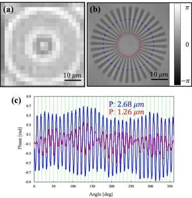
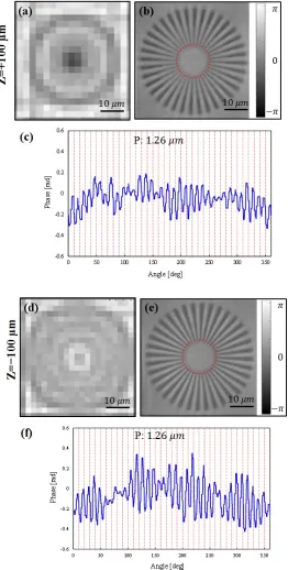
objective lens in the 1:1 imaging configuration. Because the main sample of the EmSight Figure 3.7: Digital refocusing of the EmSight. (a-c) 100 , and (d-f)
[image:57.612.198.460.88.606.2]slide glass using FIB (Focused Ion Beam). The largest and smallest periodicity is 4 µm and 1 µm, respectively, and the depth of the etched surface is about 230 nm. The raw intensity image and the FPM reconstructed phase image of the sample are shown in Figure 3.5 (a) and (b), respectively. In Figure 3.5 (c), fully resolved line profile (blue line) and the smallest resolved line profile (red line) are shown. By imaging the sample from 169 different LED directions and combining the low resolution images using Fourier ptychographic algorithm (synthetic NA of 0.42), the resolution of the system is increased by about 4 times, resolving all the spokes of periodicity of 1.26 µm.
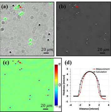
Next we used a mixture of green fluorescence beads and non-fluorescent beads (4.5 µm diameter) to check the fluorescence and FPM phase imaging performance. A raw bright field image overlaid with a fluorescence image (green color) is shown in Figure 3.6 (a). We expect EmSight users to use the fluorescence images to identify targets labeled by, or expressing specific fluorophores, and FPM reconstructed higher resolution images to compensate for the diffraction-limited fluorescence image of the targets. For simplicity, we did not apply resolution improving methods to the fluorescence imaging in the current EmSight design, however, we note that the resolution of the fluorescence images may be enhanced by adopting special illumination methods such as patterned illumination or scattering illumination [46] or aberration correcting methods [17] for those applications requiring higher-resolution fluorescence imaging. As shown in Figure 3.6 (a), the fluorescence beads are clearly distinguishable from the non-fluorescent beads by the fluorescence signal. Two beads that are attached to each other (labeled with red arrow) are resolved from the FPM reconstructed intensity (Figure 3.6 (b)) and phase (Figure 3.6 (c)) images, and the fluorescence image (Figure 3.6 (a)) gives us information on which bead is fluorescent amongst them.
∙
∆ , (3.1)where T is the thickness of the bead, λ is the wavelength of the light, Δϕ is the phase relative to the background phase, and Δn is the refractive index difference between the sample and the background. In Figure 3.6, the polystyrene beads (n=1.58) are immersed in oil (n=1.515) and green LEDs (530 nm) are used for illumination. The converted line profile indicated in Figure 3.6 (c) is shown in Figure 3.6 (d). The measured curve closely matched the expected profile of an ideal sphere, which indicates the FPM reconstructed phase information of the EmSight is quantitatively accurate. We note that there are small asymmetries in the phase of some beads in Figure 3.6 (d). These small asymmetries can be attributed to the abrupt phase change of boundary between the bead and surrounding oil.
Digital refocusing is one of the most important features of the FPM and it is especially useful in live cell imaging, where multi-day or multi-week experiments can be vitiated by image defocus caused by system drifts and well plate misalignments. By introducing a quadratic defocus phase term into the support constraint in the spatial frequency domain, we can digitally refocus the defocused raw images during the FPM reconstruction [9]. In order to characterize the refocusing performance of the EmSight, we intentionally image a defocused Siemens star phase target and digitally refocused the image during the FPM reconstruction (see Figure 3.7). For the depth of field (DOF) test, we built the equivalent imaging system on the optics table and used a mechanical stage for making displacement of the sample from the detection system. For the refocusing of the defocused sample, we use the angular spectrum wave propagation method [47, 48]. By the discrete sampling of the camera and the Nyquist sampling theorem, there is a maximum distance that the angular spectrum method can be applied as in Equation (3.2):
z
∆
√,
z
∆
√,
(3.2)
directions. In our system, we matched the NA of objective lens with camera pixel size, and we used 128 pixel x 128 pixel for each tile of image reconstruction, and therefore the maximum distance is calculated as Equation (3.3):
z
∆
∙
1
2
1
∙
2
128
2.2 μm ∙
. .2
1,150
. (3.3)are shown in Figure 3.8. Blurry neurites of the neurons in the defocused image are clearly refocused in the FPM reconstructed image.
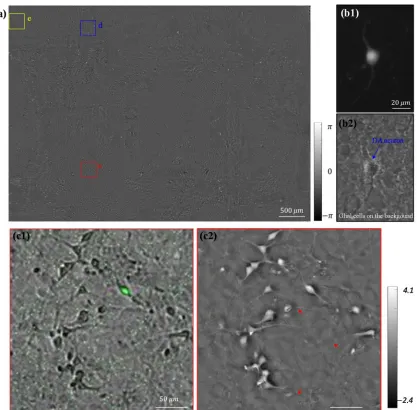
We also used the EmSight to image a mouse ventral midbrain culture sample in order to test the FOV of the system and to assess the fluorescence imaging capability of the system. The sample was fixed with paraformaldehyde (PFA) and immersed in phosphate buffered saline (PBS) for the imaging. The full FOV of one imaging unit of the EmSight is 5.7 mm × 4.3 mm, as shown in Figure 3.9 (a). This sample was originally seeded with Figure 3.9 (cont.): (c1-e1) Raw images overlaid with fluorescence images (Green color).
[image:62.612.136.515.98.444.2]Figure 3.9 (a). Images from three representative DA neurons are shown in Figure 3.9 (c-e). The eGFP fluorescence signal intensity captured from the EmSight system is strong enough to be used to identify the target DA neurons, as shown in Figure 3.9 (c1-e1). Figure 3.9 (c2-e2) show the FPM reconstructed phase images at distances of 1.8 mm, 2.2 mm, and 3.4 mm from the center of the FOV, respectively. Neurites of the neuron which are not distinguished in the raw images are clearly visible in the reconstructed phase images as indicated in red arrows. For comparison, fluorescence image and Zernike phase contrast image of a dopaminergic neuron (DA neuron) are shown in Figure 3.9 (b) using 20X/NA0.4 objective lenses. We note that the neuron sample in our experiment is a primary mixed culture and the surface of the well plate is covered with glial cells. The unevenness of the background in Figure 3.9 (c2-e2) is the image of the glial cells. These glial cells can be seen in the Zernike Phase contrast image of Figure 3.9 (b2). Also dark halos surrounding some cell bodies in the phase images are attributable to the physical
[image:65.612.160.490.99.367.2]phase contrast) are observed in the phase contrast image as well.
3.5 Live cell culture imaging
To conduct live cell imaging using the EmSight system, we cultured ventral midbrain from the GENSAT tyrosine hydroxylase (TH)-eGFP strain [49], a BAC transgenic mice line driving eGFP from the TH promoter. The cultures were grown based on the procedure we have recently established for the long-term primary culture of mouse ventral midbrain neurons [50, 51]. Each of the neuron-glia ventral midbrain cultures consisted of a glial cell monolayer, DA neurons generating TH-eGFP, and other midbrain neurons. We employed the EmSight system to image and monitor the cultures over a 3-week period.
Our ventral midbrain cultures were obtained from embryonic day 14 mouse embryos which were extracted from timed pregnant mice using a standard method [52]. The glial cells and midbrain neurons were grown in a 6-well plate and the culture medium was exchanged at three-day intervals over the 3-week imaging period. The EmSight system captured images from each well at one hour intervals for the FPM imaging. Fluorescence imaging was conducted once per day for each well. Figure 3.10 (a) shows representative FPM phase images from the time-lapse imaging of a DA neuron and midbrain neurons. The tracked DA neuron is successfully identified using the eGFP fluorescence signal and marked with a yellow circle. By comparing each subsequent image, we choose a cell having minimum position and size change with a target cell of previous time frame as a target cell of current time frame. In our one hour period time-lapse imaging, this tracking method worked well for most of cells. For the time sequences cells were moving fast, we manually corrected the tracking error. We successfully tracked the target cell for the duration of the culture experiment, and Figure 3.10 (b) shows the positional trace of the tracked target cell. Images of the entire field of view and the reconstructed FPM phase images for each of the 6 wells at culture day 7 are shown in Figure 3.11.
the time-lapse images as shown in Figure 3.12. Two putative mother cells as indicated by the red and blue arrows divided into daughter cells. These cells began dividing on approximately day 14 of culture. Such cell divisions were observed in each of the 6 wells in the plate. We think that these dividing cells may be neural stem cells or progenitor cells. 3.6 Dual channel fluorescence imaging
[image:67.612.135.513.97.453.2]sized bead) and a phase sample (HeLa cell line) are shown in Figure 1.14 and dual channel fluorescence image from sender and receiver 3T3 cells is shown in Figure 1.15. 3.7 Discussion and conclusion
We have successfully developed an incubator embedded cell culture imaging microscope (EmSight) system based on the Fourier ptychographic microscopy (FPM) method. We used two inexpensive low magnification objectives to perform 1:1 imaging of the target culture onto the imaging sensor chip. By using the FPM meth