A New PHD Algorithm in Unknown Clutter Environment Based on Box Particle

2017 2nd International Conference on Software, Multimedia and Communication Engineering (SMCE 2017) ISBN: 978-1-60595-458-5

A New PHD Algorithm in Unknown Clutter

Environment Based on Box Particle

Shuai WEI*, Xin-xi FENG and Quan WANG

Information and Navigation College of Air Force Engineering University, Xi’an, Shaanxi 710077, China

*Corresponding author

Keywords: Multi-target tracking, Probability hypothesis density, Interval analysis, Box particle, Unknown clutter.

Abstract. In unknown clutter environment, traditional Probability Hypothesis Density (PHD) filter in multi-target tracking cannot guarantee a good performance and multitude number of particles leads to time consuming and low efficiency. Aiming at the problems, a new PHD filter tracking algorithm in unknown clutter environment based on interval analysis was proposed. Firstly, radar targets and clutter disjoint union state space modeled were established in random finite set. Next, using measurement model set up clutter model and derived to multi-target updated state function based on box particles. Additionally, the state of multi-target was recursively estimated in utilization of PHD filter box particles. Simulation reveals that the proposed algorithm is able to dramatically lower computational time with better tracking performance compared with traditional box particle filter.

Introduction

The traditional multi-target tracking algorithms need data association[1], leading to a large workload. So, Mahler proposed the theory of Random Finite Set (RFS) to solve the problem of unknown and variable number of targets, reducing the computational complexity and ensuring the tracking accuracy[2].

The traditional PHD filter establishes the clutter intensity _k

 

z as a known Poisson

distribution process[2]. But in reality, the clutter estimation and analysis will increase the time-consuming. In [3], the clutter was assumed to time-varying parameters, and estimated at each

step. [4] and [5] used the Rayleigh distribution and



distribution to make the clutter model

respectively. In [6], it proposed a finite hybrid model to describe the density function of the clutter and estimated with Markov chain Monte Carlo algorithm [7]. In [8], the clutter model was estimated using joint state of target and clutter. In [9], it assumed that the multi-target tracking model obeys the Poisson process. In [10] [11], with an unknown prior knowledge, the estimation of the clutter led to a high complexity and much time-consuming.

So we introduce the interval analysis technique, and propose the PHD algorithm based on box particle filter in unknown clutter state.

Spatial Model Establishment

Consider the establishment of mixed space model for algorithm implementation. Defined as follows:



 X



where,  denotes the mixed space, X denotes the target state space and  denotes the clutter

PHD Filtering Algorithm Based on Interval Analysis in Unknown Clutter Environment

The traditional algorithm SMC-PHD [2] and SMC-NPHD algorithm in [11] will cause a significant increase in the amount of computation. So we propose Box-SMC-NPHD to promote the algorithm efficiency.

(1) Initialization

At time k-1, there is a set of weighted box particles



( )_{, 1}  _{, 1}



1

1

,[ ] k

L i i

P k P k i w _{ } 



x to prevent new target

producing a large number of newborn particles. According to the previous measurement random set

1

k

Z , the number of new particles will denotes:

 



, , / 1 , 1, 1

i

k k k k

L_ _L_ m_ j …,m _ (1)

where, m_k₁ denotes measurements number at time k-1, and x denotes upper integer symbol.

It is generally assumed that the new target is usually present in the measurement position, with a set of uniformly distributed probability density functions, there will be:

 





 

 

, , 1 , 1 | k i k L i k U L     _{ }      



x

x z x (2)

where, _x_ i_,k_ denotes box particles of target states, _{ }

 

, i k U      x 

x denotes uniform distribution of

  , i k   

x . And the weight of newborn particle is followed by:

 

 

( )

, , / , , , ,

i

k k k k k

w_  p_ x L_ iL …，L_ (3)

where, p_,k

 

 

x denoted the newborn target probability. The initialized box particle state set consists of the previous momentary surviving part and the newborn part, which is:







 



1



 



,

( ) ( ) ( ) ( )

1 1 , 1 , 1 , 1 , 1

1 1 1

,[ ] k ,[ ] k ,[ ] k

L L

L

i i

i i i i

k k P k P k k k

i i i

w _{ } w _{ }  w_{   } 

   

x x x (4)

And the total number of particle will be L_k L_k1L_,k.

(2) Target PHD prediction

Assume the posterior intensity at time k-1 will be:

 

 

 

1 1 ( ) 1 1 k i k L i k k i

v w U

          



x

x x (5)

So the predicted intensity can be:

 

 

 

 

 

, 1

, , | 1

( ) ( )

| 1 , | 1 ,

1 k k i i k P k k

k L L

i i

k k P k k k

i i L

v w U w U

                     







x x

x x x (6)

The weight expression of newborn particle can be:

 

 





 





,

( )

, , / _k , |

i i

i

k k k k k k

w  x L b_ x Z (7)

(3) Clutter intensity prediction

 

 





1



 



,



 



( ) ( )

| 1 1| 1 | 1 , | 1 | 1 , | 1 , | 1 ,

1 | | | [ ] k k k L L i i i i

k k k k k k P k k k k P k k k k k k

i L

v v p w p w p

                    

 



_x _ 



x

(4) Target update

The predicted intensity at time k can be:

 

 

 

| 1

| 1

( )

| 1 | 1

1 k k i k k L i

k k k k

i

v w U

           



x x x (9) The update intensity can be

 

 

 

| 1 ( ) 1 k k i k L i k k i

v w U

        



x x x (10) The update weight can be:

 







 





 

 



 





 

| 1



 



,k | 1 | 1

( ) ( )

| 1 ,k | 1

0 ( )

, | 1 , | 1 | 1

1 | 1 | k k k i i

D k k k k k

i

i i

k k k D k k L

z i i

D K k k k k z k k k k

i

p g

w w p

p g  v   w

                     _  _{ }      _{  } 





Z

x z x

x

z x

(11) (5) Clutter intensity update

   



 



 







 



 





 

 

 

0

,k | 1

0

| 1 ,k | 1 0

, | 1

| 1

| k

i

D k k k

i

k k k D k k

z D K k k k k

p g

v v p

p g v C

               _  _{ }  _  _{ }  _  



Z x z x z z (12) (6) Constraint box particles

The purpose of constraining box particles is to directly remove the area without overlapping. The measurement likelihood of box particle at time k can be:

 

 







 

 



 

| 1 | 1

| i i , /

k k k cp k k

g z x      h x   z x

(13)

 

 



| 1 ,



i

cp k k h     

  x  z denotes the rule to constraint and gets to the new box particle.

(7) Estimation

The number estimation can be:

1 ,

( )

1

ˆ _int Lk L k i

k k i L w       _{ }





 ₍₁₄₎

where, int

 

 denotes integer rounding symbol.

(8) Resampling

Assume L_k represents the number of box particle resampling. Divide the box particles

according to the number of copies of the box particles and normalize the weights. The set of box

particle will be



 _, ( )_,



1

[ ], 1/ k

L

i i

P k P k k

i

w L





x

(9) Target state extraction

The particles are clustered by K-means algorithm and the target state is obtained from the clustering center. Select the particle with the weight greater than a certain threshold, and get the expression of the target state estimate, i.e.

 





( )

, [ , ] , 1, 2, , ˆ

i i

j P k P k k

i

s 



w mid x j  L

Numeral Studies

In order to verify the effectiveness and feasibility of the algorithm, we compared algorithms of SMC-PHD, SMC-NPHD and the proposed Box-SMC-NPHD.

Parameters

Four moving targets are tracked in the monitoring area and are uniformly linearly moved. The

monitored area is [-150,200]m×[-150,200]m, time interval T_s is 1s, whole time processing is 30s.

target states are represented by x



x x y y, , ,



T. And



x y,



denotes the position and



x y,



denotes the velocity. The target state equation is followed x_k Fx_k1Γw_k , where

1 ,

0 1

s T

   

_{ } _{ }

   

Α 0

F Α

0 Α . Process noise variance is Qk diag



0.5 0.5



, the state noise input matrix is

T ₂

, 2

s s

T T

 

 

_{    }

   

Β 0

Γ Β

0 Β

, and the initial states of target are x1 



50,9, 40, 11 



T,





T 2 25,8, 40,10

x ,





T

3 10, 7, 75,9

x , x₄ 



100, 7, 150,10



T. And target 1 has a duration of 1 to 8 seconds, target 2

has a duration of 7 to 20 seconds, target 3 has a duration of 12 to 35 seconds, target 4 has a duration of 28 to 40 seconds.

The system measurement equation is z_k Hx_kv_k, where 1 0 0 0

0 0 1 0

 

  

 

H , and measured noise

variance is



2 2



2.5 , 2.5 diag  

 _{ }

R , interval measurement applies to

 

_k

 

_k 0.6 , _k

 

_k 0.4

k h    h   

z x v x v where  



21, 25



T, detection probability pD k, 0.98,

survival probability p_s,k 0.95, newborn probability p,k 0.01.

The clutter is uniformly distributed in the observed area, and the number of measured clutter is

expressed as the mean 



of the Poisson distribution. A denotes the monitoring area and

denotes clutter intensity. Clutter detection probability p_d0 0.3 , newborn probability





| 1 | 0.05

k k

p   x  . And the state box particles has the interval values are 6m, 7m and the speed of

1m / s.

Results and Analysis

[image:4.595.209.382.606.741.2]

Choose optimal sub-mode distribution (OSPA) as the evaluation criterion. Select the parameter c = 50, p = 2. For each interval, the number of continuous particles is 2000, the number of new particles is 50, the number of continuous particles is 40, and the number of new particles is 1. The simulation carried out 100 Monte Carlo experiments were respectively, and the running time results were analyzed. Interval analysis tools use the INTLAB toolbox.

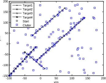
Figure 1. Target trajectory and interval measurement with clutters.

Figure 1 shows the four trajectories of the targets in a clutter environment. The clutter density

values are 3×10-5, 1.5×10-4, 3×10-4 respectively. Assume that the clutter density remains

-100 -50 0 50 100 150 200

-150 -100 -50 0 50 100 150 200

x/m

y/

m

substantially constant over the time interval in which the tracking is performed.

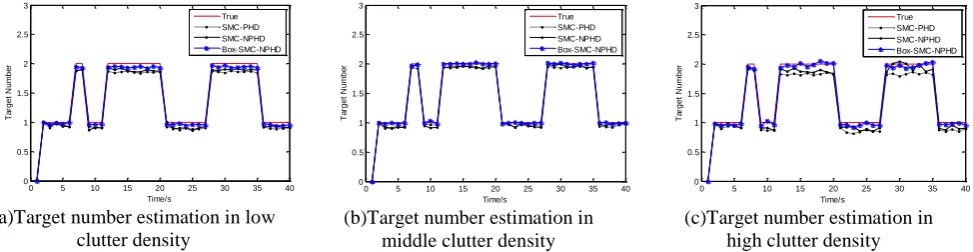
It can be seen from Figure 2 (b), the three algorithms can estimate the number of targets better because the medium clutter density is matched with the traditional PHD filter prior clutter model.

In comparison with Figure 3, the OSPA mean of the first two is basically the same, but at high density clutter, the former is 5.81% lower than the latter. This is because the high density clutter environment is a more pronounced inaccurate measurement.

(a)Target number estimation in low clutter density

(b)Target number estimation in middle clutter density

[image:5.595.63.550.159.285.2]

(c)Target number estimation in high clutter density

Figure 2. Three filter simulation comparison on target number estimation in different clutter situations.

(a)OSPA distance in low clutter density

(b)OSPA distance in middle clutter density

[image:5.595.68.545.308.413.2]

(c)OSPA distance in high clutter density

Figure 3. Three filter simulation comparison on OSPA distance in different clutter situations.

[image:5.595.186.407.596.659.2]

Table 1 shows the complexity of the three filtering algorithms. It can be seen that the SMC-NPHD is about 20% more than the SMC-PHD, while the box-SMC-NPHD based on the interval analysis is about 1/6 of the SMC-NPHD run time. This is because the number of box particles required for this improved algorithm is much smaller than the remaining two particle filter algorithms. The latter two algorithms based on particle filtering require 2050 particles, because the number of new particles to capture new targets, resulting in a large number of time consumption. Although the improved algorithm based on box particle filtering can take part of the time in interval analysis, only 41 boxes of particles can achieve similar precision to the particle filter algorithm. The large number of particles is reduced so that the algorithm achieves the running time of the significant reduction, thus improving the timeliness and applicability.

Table 1. Three filters comparison on complexity in different clutter situations.

Clutter Intensity

Time/s

PHD NPHD Box-NPHD

3×10-5 15.453 18.516 2.954

1.5×10-4 17.152 20.583 3.287

3×10-4 19.038 23.243 3.976

Conclusion

In this paper, a PHD algorithm based on box particle filtering in unknown clutter environment is proposed. The algorithm uses the box particle weighting method to establish the unknown clutter model by measurement data, derive the target state updating equation, and recursively estimate the target state with box particle PHD filter, which greatly reduces the number of required particles. The simulation results show that the algorithm can effectively reduce the computation time of the algorithm while ensuring the target tracking performance compared with the multi-target particle filter algorithm when the clutter environment does not match the prior model.

0 5 10 15 20 25 30 35 40 0

0.5 1 1.5 2 2.5 3

Time/s

T

a

rg

e

t

N

u

m

b

e

r

True SMC-PHD SMC-NPHD Box-SMC-NPHD

0 5 10 15 20 25 30 35 40 0

0.5 1 1.5 2 2.5 3

Time/s

T

a

rg

e

t

N

u

m

b

e

r

True SMC-PHD SMC-NPHD Box-SMC-NPHD

0 5 10 15 20 25 30 35 40 0

0.5 1 1.5 2 2.5 3

Time/s

T

a

rg

e

t

N

u

m

b

e

r

True SMC-PHD SMC-NPHD Box-SMC-NPHD

0 5 10 15 20 25 30 35 40 0

20 40 60 80

Time/s

O

S

P

A

/m

SMC-PHD SMC-NPHD Box-SMC-NPHD

0 5 10 15 20 25 30 35 40 0

20 40 60 80

Time/s

O

S

P

A

/m

SMC-PHD SMC-NPHD Box-SMC-NPHD

0 5 10 15 20 25 30 35 40 0

20 40 60 80

Time/s

O

S

P

A

/m

Acknowledgement

This research was financially supported by the National Science Foundation (61571458).

References

[1] C. Hue, J.L. Cadre, P. Perez. Sequential Monte Carlo methods for multiple target tracking and

data fusion[J]. IEEE Transactions on Signal Processing, 2002, 50(2): 309-325.

[2] Mahler R. Statistical Multi-source multi-target Information Fusion[M]. Boston: Artech House

Publishers, 2007.

[3] B.T. Vo, B.N. Vo, A. Cantoni. Analytic implementations of the cardinalized probability

hypothesis density filter[J]. IEEE Transactions on Signal Processing. 2007,55(7): 3553-3567.

[4] D. Musicki, M. Morelande, B. L. Scala. No parametric target tracking in non-uniform clutter.

The 8th International Conference on Information Fusion[C]. Philadelphia, USA, 2005, 1-6.

[5] M. G Rutten, N. J. Gordon, S. Maskell. Recursive track-before-detect with target amplitude

fluctuations[J]. IEEE Proceedings: Radar, Sonar and Navigation. 2005,152:345-352.

[6] Lian Feng, Han Chongzhao, Liu Weifeng. Estimating Unknown Clutter Intensity for PHD

Filter[J]. IEEE Transactions on Aerospace and Electronic Systems, 2010,46(4):2066-2078.

[7] Vo B N, Singh S, Doucet A. Sequential Monte Carlo methods for multi-target filtering with

random finite sets[J]. IEEE Transactions on Aerospace and Electronic Systems, 2005,41(4): 1224-1245.

[8] Mahler R, Vo B T, Vo B N. CPHD Filtering with Unknown Clutter Rate and Detection

Profile[J]. IEEE Transactions on Signal Processing, 2011,59(8):3497-3513.

[9] Streit R. Poisson Point Processes: Imaging, Tracking, and Sensing[M]. Heidelberg: Springer,

2010.

[10]Schikora M, Gning A, Mihaylova L, et al. Box-particle Intensity Filter[C]. 9th IET Data Fusion

and Target Tracking Conference. Stevenage: IET, 2012: 1-6.

[11]Li Cunyun, Jiang zhou, Ji Hongbing. Novel PHD filter in unknown clutter environment [J].