2016 International Conference on Computational Modeling, Simulation and Applied Mathematics (CMSAM 2016) ISBN: 978-1-60595-385-4
Estimating Lorenz Curve of Income by Cubic Spline with Multiple Knots
Ying LIANG
1, Han YANG
2,*, Jia-xu ZHANG
2, Qiang LI
2and Xue-zhang LIANG
21
Business School of Jilin University, Changchun, 130012, P.R. China
2
Mathematics School ofJilin University, Changchun, 130012, P.R. China
*Corresponding author
Keywords: Cubic spline with multiple knots, Linear programming, Aggregated Lorenz curve, Gini index.
Abstract. In this paper we propose a method for convex approximation of the Lorenz curve by cubic-spline with multiple knots. This method is applied to the China-2005 grouped data of urban and rural residents’ income, published in “China Statistical Yearbook-2006”. Then, we use the method proposed in this paper to estimate the Lorenz curves and the Gini index of urban and rural residents’ income in China, respectively. Finally we estimate the Lorenz curve of residents’ income of whole China (2005) by the aggregated approach.
Introduction
The Lorenz curve and the Gini index are important tools for analyzing the distribution of income and the degree of wealth distribution inequality. On the basis of the known grouped data of income, there are a variety of methods to approximate the Lorenz curve [1-5]. In this paper we present a method to approximate the Lorenz curve convexly by cubic-spline with multiple knots. We apply the method to China-2005 grouped data of urban and rural residents’ income, published in “China Statistical Yearbook-2006” [6], to approximate urban and rural income Lorenz curves respectively. Furthermore, we obtain the Lorenz curve of whole China(2005) by the aggregation approach[7].
The Lorenz curve is a monotonously increasing convex curve on [0,1]and satisfiesL(0)=0,L(1)=1. In this paper, the income distribution function, it’s inversion and density function are respectively denoted as
) (x F
p= , (1.1)
) ( )
(p F 1 p x
x= = − , (1.2)
and
dx dp x F x
f( )= '( )=
, (1.3) where x represents income and p represents cumulative population share, with
) , 0 [ ∞ ∈
x andp∈[0,1].
Average income has the following expression:
∫
∫
=∞=
0 1
0
) ( )
(pdp xf x dx x
µ
∫
∫
= = = x p dt t tf dq q x p L L 0 0 ) ( 1 ) ( 1 ) ( µµ (1.5)
and ) ( 1 ) (
' p x p
L dp dL µ = = (1.6) Obviously, we have:
) ( )
(p L' p x
x= =
µ
(1.7)The rest of this paper is organized as follows. In section 2,we introduce a new method of estimating Lorenz curve convexly by cubic-spline with multiple knot. In section 3, we briefly describes the aggregation formula. Section 4 provides the Lorenz curves of urban and rural area in China (2005) by the method proposed in section 2 ,and estimates the Lorenz curve of whole china(2005) by aggregation of the Lorenz curves of urban and rural area in China (2005). Concluding remarks is presented in section 5.estimates
A Kind of Approximation of Cubic Spline with Multiple Knots
Assume that
{ }
xi ni=1is a set of real nodes satisfying0=x1<<xn=1ands(x)is continuous functionon [0,1]. We call s(x) a cubic spline with multiple nodes
{ }
xi in=1 on [0,1][8], if the function s(x) has a first-order continuous derivative on [0,1] and equates to a real algebraic polynomial of degree ≤ 3 in each interval [xj,xj+1] (j=1,…,n-1).Let L=L(p) be a given Lorenz curve, and
{
(Xi,Yi)}
im=1 be the grouped data of the Lorenz curve ,which satisfy Yi =L(Xi) (i=1,2,,m) ,with 0=X1<X2<<Xm =1 and1 0=Y1 <Y2 <<Ym = .
We try to approximate the Lorenz curve L(p) by cubic splines(x)with multiple knots
{ }
xi in=1on[ ]
0,1 satisfying{ }
Xi mi=1 ⊆{ }
xi ni=1 and m≤n (We call thes(x) a spline representation of L(p) ). Assume that xk Xjj = (j=1,...m) with 1=k1<k2 <<km−1<km =n and the corresponding
values of spline function s(x) in the knots are
{ }
yi ni=1 (0≤ yi≤1),and the first derivatives are{ }
ni i
y' =1.Then, in each interval[xj,xj+1] (j=0,1,…,n-1), referring to cubic Hermite interpolation formula [9] , the spline functions(x) has the following expressions:
+ − − + − − − + − − + = + + + + 2 2 1 2 1 1 2 2
1 ( )
) ( ' ) ( ) ) ( 2 1 ( ) ( ) ) ( 2 1 ( ) ( i i i i i i i i i i i i i i i h x x x x y h x x h x x y h x x h x x y x s 2 2 1 1 ) ( ) ( ' i i i i h x x x x
y+ − + −
, (2.1) and the second derivative of si(x)has the following expression :
+ − − − = + + 3 1 1 '' ) 2 ( 6 ) ( i i i i i i h y y x x x x
s 22[ i'(2 − i −2 i+1)+ i'+1(3 −2 i − i+1)]
i x x x y x x x y
h , (2.2)
Becausesi''(x) is a liner function on [xi,xi+1], si''(x)≥0 on [xi,xi+1]if and only if si''(xi)≥0and 0 ) ( 1 '' ≥ + i i x
s .Therefore,s(x) is a monotone increasing and smooth convex curve on [0,1] if and only if the following inequalities hold
) 1 1 ( 0 1 1 3 1 3 2 1 ' 1 ' − ≤ ≤ ≤ − +
+ + y+ i n
h y h y y i i i i i i , (2.3) ) 1 1 ( 0 1 1 3 2 3 1 1 ' 1 ' − ≤ ≤ ≤ + − −
− + y+ i n
h y h y y i i i i i i .
Then, the formula of Gini index corresponding to s(x) is
∫
= 1 0 ) ( s 2 -1G p dp
, (2.4) where
+ + =
∑
∫
2 = ( + )1 ) ( 1 1 1 0 n
i hi yi yi
dp p
s
∑
= + +
n
i1hi yi yi ' ' 1 2 ) ( 12 1
. (2.5) Obviously, as definite integral in formula(2.5) reaches the minimum value, the Gini index reaches the maximum value. Assume
C= + +
∑
= ( + ) 2 1 1 1 ni hi yi yi
∑
= + +n
i1hi yi yi ' ' 1 2 ) ( 12 1
. (2.6) The problem of estimating Lorenz curve of income by using cubic-spline with multiple knots can be transformed to the question of solving the linear programming as following:
Minimize the objective function C subject to the following constraint:
) 1 -n , 1,2, ( 0 1 1 3 1 3 2 1 ' 1 ' = ≤ − +
+ + y+ i
h y h y y i i i i i i i n Y y =
i (i=1,2,,m) (2.7)
1) -n , 1,2, ( 0 1 1 3 2 3 1 1 ' 1 ' = ≤ + − −
− + y+ i
h y h y y i i i i i i .
We solve the above linear programming problem with the simplex (Big-M)method [10] to obtain yi
and and yi' (i=1,2,,n ) .Furthermore, we can obtain the Lorenz curve by using the Hermite interpolation formula (2.1) in each interval [xi,xi+1].
Next, we introduce the methods for selecting urban and rural spline node
{ }
xi ni=1 respectively. Assume that there are m1 sets of the given grouped data of urban residents’ income, spline nodes{ }
n i ii
x =Xi i=1,2,3.
4
x =(X3+X4) 2
) (
1
-X 3 4 3
4 ) 1
(i− +j+ = i+ + i+ − i+
k X X
k j
x ( )
i=1, 2, 3; j=1,2,...,k. (2.8)
. 3 , 2 , 1 ,
6 3 k 3
2+ + =X + i=
x i i
. 2 , 1 , 2 / )
( 3 2
5 2
3 + 1+ − = X 1+− +X 1+− i=
x k m i m i m i
where hi=xi+1−xi (0≤i≤n−1),then the number of spline nodes is n= 3k+m1 with m1=9and 4
k = in section 4.
Assume that there are m2 sets of the given grouped data of rural residents’ income, and rural spline
nodes
{ }
xi ni=1 of estimating Lorenz curve for rural area can be expressed as following:, ) )(
1
( 1
1
( X j x x k
xi−)k+j = i+ − i+ − i i=1,2,,m2−1 ; j=1,2,...,k.
m
n X
x =
(2.9) where hi =xi+1−xi (0≤i≤n−1) ,then the number of spline nodes is n=( (m2−1)k +1 with
5
2 =
m and k =3in section 4.
Aggregation Formulas for Lorenz Curve
Assume that the population of urban and rural area are P1 and P2respectively, the total population is P . The ratio of urban and rural population to nation are represented asλ1=P1 Pandλ2=P2 P respectively, obviously,λ1+λ2 =1. Let µ1 be the average of urban residents’ income and µ2 be the average of rural residents’ income.
Distribution function ,density function and Lorenz curve of urban income are defined as,
) (
p1= F1 x , f1(x)= F1'(x), and L1 = L1(p1). (3.1)
Distribution function ,density function and Lorenz curve of rural income are defined as,
2
p =F2(x), f2(x)=F2'(x), and L2 =L2(p2). (3.2)
And nationwide Lorenz curve is defined as,
) (p L
L= . (3.3)
Then, the aggregation formula[7] is as following:
2 2 1
1p p
p=λ +λ
) ( )
( )
( 1 1 '2 2 2
'
1 p L p L p
L
x=
µ
=µ
=µ
(3.4))] ( )
( [ 1 )
(p 1 1L1 p1 2 2L2 p2
L λµ λ µ
µ +
=
,
µ λ µ λ
µ= 1 1+ 2 . (3.5)
Based on the spline representations of Lorenz curve L(1 p1) and L2(p2), we can obtain the values
of L(p) by aggregation formula(3.4) for given p (0≤ p≤1).
A Practical Application
The method described in section 2 is applied to the grouped data of urban and rural area in China(2005) ,published in "China Statistical Yearbook (2006)"[6] , we obtain the Lorenz curve of urban and rural area. Furthermore we get the Lorenz curve of whole China(2005) by aggregation approach. In the process of calculation, income of urban residents adopts disposable income, rural residents' income adopts net income. The average income of urban residents is µ1=10483, the average income of rural residents is µ2=3254.9 and λ1=0.4299, λ2=0.5701. The grouped data of
urban and rural China are as following Tables 1and 2.The calculation results are as following Table 3 to 9.
Table 1. The grouped data of residents’ income in urban China (2005).
X 0.0000 0.0559 0.1115 0.2205 0.4311 0.6319 0.8201 0.9115 1.000 0 Y 0.0000 0.0131 0.0329 0.0830 0.2160 0.3897 0.6140 0.7605 1.000 0
Table 2. The grouped data of residents’ income in rural China (2005). X 0.000 0 0.2258 0.4384 0.6397 0.8292 1.0000 Y 0.000 0 0.0721 0.2017 0.3742 0.6042 1.0000
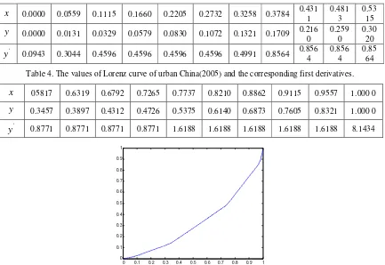
Table 3. The values of Lorenz curve of urban China(2005) and the corresponding first derivatives.
x 0.0000 0.0559 0.1115 0.1660 0.2205 0.2732 0.3258 0.3784 0.431 1
0.481 3
0.53 15
y 0.0000 0.0131 0.0329 0.0579 0.0830 0.1072 0.1321 0.1709 0.216
0
0.259 0
0.30 20
'
y 0.0943 0.3044 0.4596 0.4596 0.4596 0.4596 0.4991 0.8564 0.856 4
0.856 4
[image:5.612.92.525.408.706.2]0.85 64 Table 4. The values of Lorenz curve of urban China(2005) and the corresponding first derivatives.
x 05817 0.6319 0.6792 0.7265 0.7737 0.8210 0.8862 0.9115 0.9557 1.000 0
y 0.3457 0.3897 0.4312 0.4726 0.5375 0.6140 0.6873 0.7605 0.8321 1.000 0
'
y 0.8771 0.8771 0.8771 0.8771 1.6188 1.6188 1.6188 1.6188 1.6188 8.1434
0 0.1 0.2 0.3 0.4 0.5 0.6 0.7 0.8 0.9 1
0 0.1 0.2 0.3 0.4 0.5 0.6 0.7 0.8 0.9 1
Table 5. The values of Lorenz curve of rural China (2005)and the corresponding first derivatives.
x 0.0000 0.0749 0.1499 0.2248 0.2960 0.3672 0.4384 0.5055 0.5726 0.6397 y 0.0000 0.0000 0.0266 0.0721 0.1153 0.1585 0.2017 0.2424 0.2950 0.3742
'
[image:6.612.148.465.165.374.2]y 0.0000 0.0000 0.6067 0.6067 0.6067 0.6067 0.6067 0.6067 1.1362 1.2032 Table 6. The values of Lorenz curve of rural China (2005) and the corresponding first derivatives.
x 0.7029 0.7660 0.8292 0.8861 0.9431 1.0000
y 0.4502 0.5262 0.6022 0.6707 0.7392 1.0000
'
y 1.2032 1.2032 1.2032 1.2032 1.2032 11.3360
0 0.1 0.2 0.3 0.4 0.5 0.6 0.7 0.8 0.9 1
0 0.1 0.2 0.3 0.4 0.5 0.6 0.7 0.8 0.9 1
Figure 2. Estimation of Lorenz curve for rural China(2005).
Table 7. The values of Lorenz curve of whole China (2005) and the corresponding first derivatives.
x 0.0000 0.1000 0.2000 0.3000 0.4000 0.5000 0.6000 0.7000 0.8000 0.9000 y 0.0000 0.0118 0.0428 0.0739 0.1241 0.1856 0.2492 0.3300 0.4709 0.6476
'
[image:6.612.90.522.420.706.2]y 0.0000 0.3102 0.3102 0.3156 0.6146 0.6151 0.7575 1.2533 1.4456 2.6680 Table 8. The values of Lorenz curve of whole China (2005) and the corresponding first derivatives.
x 0.9100 0.92 0.93 0.94 0.9500 0.9600 0.9700 0.9800 0.9900 1.0000 y 0.6743 0.7010 0.7277 0.7544 0.7810 0.8077 0.8344 0.8660 0.9121 1.0000
'
y 2.6680 2.6680 2.6680 2.6680 2.6680 2.6680 2.6933 3.7791 5.5405 13.4214
0 0.1 0.2 0.3 0.4 0.5 0.6 0.7 0.8 0.9 1 0
0.1 0.2 0.3 0.4 0.5 0.6 0.7 0.8 0.9 1
Table 9. The estimations of rural , urban and nationwide Gini index in China(2005). year Urban Gini index Rural Gini index nationwide Gini index
2005 0.3468 0.3911 0.4843
Conclusion
From the above computation results, we can see that Lorenz curve obtained by cubic-spline with multiple knots not only keeps monotonicity and convexity of the Lorenz curve, but also has better approximation performance. Table 9 shows that nationwide Gini index of China (2005) calculated by this paper is very close to 0.485 , reported by National Statistical Bureau in 2014. Obviously, the approach proposed in the paper is feasible and effective. The results reported in tables 7 and 8 have some reference value
Acknowledgement
This research was financially supported by the Chinese National Science Foundation ( No.11271041) , Jilin University Philosophy and Social Science Fund(2011QY093), and China Scholarship Council (CSC).
References
[1]Jospesh L. Gastwirsh, Mariacia Glauberman, The interpolation of the Lorenz curve and Gini index from grouped data, Econometrica,Vol. l44, No.3 (1976) 479-483.
[2]Yan Jie-li, Wang Zu-xiang. Review and recent progress in the research of Lorenz curve model, Statistics & Decision, No. 1 (2014) 34-39. (Chinese)
[3]Dagum C. , A New Approach to the Decomposition of the Gini Income Inequality Ratio , Empirical Economic, 22 (1997) 515-531.
[4]Chotikapanich D., et al., Estimating Income Inequality in China Using Grouped Data and the Generalized Beta Distribution, Review of Income and Wealth, 53 (2007) 127-147.
[5]Wang ZX, et al., A General Method for Creating Lorenz Curves. Reviews of Income and Wealth (2011) 561-582.
[6]Nationl Bureau of China, China Statistical Yearbook, China Statistics Press, 2006.
[7]Ying Ling, Jiaxu Zhang, Dandan Jia ,et al., Estimating Lorenz Curve of Income in China by Cubic Spline Interpolation. Research & Reviews: Journal of Statistics and Mathematical Sciences Vol.1, No. 2, (2015) 36-39.
[8]De Boor C., A Practical Guide to Splines, New York. Springer-Verlig, 1978.
[9]Zhou Yun-shi, Liang Xue-zhang, Chang Yu-tang. Ma Fu-ming. Numerical analysis[M]. Heigher Education Press, 2008. (Chinese).