Pricing and Hedging Exotic Options in Stochastic
Volatility Models
Zhanyu Chen
Supervised by Prof. Thorsten Rheinl¨ander, Dr. Angelos Dassios The London School of Economics and Political Science
A thesis submitted for the degree of Doctor of Philosophy
Declaration
I certify that the thesis I have presented for examination for the MPhil/PhD degree of the London School of Economics and Political Science is solely my own work other than where I have clearly indicated that it is the work of others (in which case the extent of any work carried out jointly by me and any other person is clearly identified in it). I confirm that Section 3.2 was jointly co-authored with Prof. Elisa Al`os and Prof. Thorsten Rheinl¨ander.
Acknowledgment
First of all, I would like to express my gratitude to Prof. Thorsten Rheinl¨ander for his guidance, support, patience and encouragement throughout my doctoral studies. On one hand, he left me all the freedom I wanted, encouraging and developing me to carry out the independent research. On the other hand, whenever I needed help, he was always there to share his knowledge and technical advices to guide me through the problems, which was essential to the completion of my thesis. I also want to thank for his warm hospitality during my stays at Vienna University of Technology.
My sincere thanks go to Dr. Angelos Dassios. He gave me all the support and advices I needed and readily accepted to supervise me after Thorsten left LSE to teach at Vienna University of Technology.
I am grateful to Jiawei Lim and Yang Yan for all the discussions and help during my study.
And my gratitude goes to my Ph.D. examiners Prof. Peter M¨orters and Dr. Hao Xing, for their reading and all the advices on my thesis.
I also want to thank Dr. Umut Cetin, Prof. Mihail Zervos, Dr. Kostas Kardaras, Dr. Erik Baurdoux, Prof. Pauline Barrieu, Ian Marshall and many other staff and colleagues at London School of Economics for helping my research in various ways.
Financial support from the London School of Economics and Political Science is gratefully acknowledged.
Abstract
This thesis studies pricing and hedging barrier and other exotic options in continuous stochas-tic volatility models.
Classical put-call symmetry relates the price of puts and calls under a suitable dual market transform. One well-known application is the semi-static hedging of path-dependent barrier options with European options. This, however, in its classical form requires the price process to observe rather stringent and unrealistic symmetry properties. In this thesis, we provide a general self-duality theorem to develop pricing and hedging schemes for barrier options in stochastic volatility models with correlation.
A decomposition formula for pricing barrier options is then derived by It¯o calculus which provides an alternative approach rather than solving a partial differential equation problem. Simulation on the performance is provided.
Contents
1 Introduction 6
1.1 Thesis Subject . . . 6
1.2 Overview of the Literature . . . 7
1.2.1 Put-call Symmetry and (Quasi) Self-duality . . . 7
1.2.2 Decomposition of option price . . . 8
1.2.3 Reflection principle and pricing exotic options . . . 8
1.3 Contribution and Organization of this Thesis . . . 8
2 General self-duality 10 2.1 Introduction . . . 10
2.1.1 Overview of the method . . . 11
2.2 Self-duality and semi-static hedging . . . 12
2.3 Generalized self-duality . . . 14
2.3.1 Standing assumption . . . 15
2.3.2 General self-duality . . . 17
2.4 Application to barrier options . . . 21
2.4.1 General results . . . 21
2.4.2 Double Barrier options . . . 24
2.4.3 Sequential Barrier options . . . 26
3 A decomposition approach of pricing and hedging barrier options 28 3.1 Introduction . . . 28
3.2 A decomposition of option prices . . . 29
3.2.1 An approximation formula for option prices . . . 32
3.3.2 Stein & Stein model . . . 41
3.3.3 Heston model . . . 44
3.4 Numerical simulation . . . 45
3.4.1 Hull and White model . . . 46
3.4.2 Stein & Stein model . . . 49
3.4.3 Heston model . . . 52
3.5 Application in hedging barrier options . . . 56
3.5.1 Overview of the method . . . 56
3.5.2 Numerical simulation . . . 57
4 Reflection principle and application on pricing exotic options 64 4.1 Introduction . . . 64
4.2 Time-changed Brownian motion and reflection principle . . . 65
4.3 Derivation of the joint density . . . 67
4.4 Closed-form valuation formula . . . 67
4.4.1 Valuation formula for zero correlation and zero interest rate. . . 67
4.4.2 Valuation formula in the general model . . . 72
4.4.3 The density for R0T Vsds and VT in the Heston model . . . 80
4.5 Numerical Simulation . . . 87
A Proof of Remark 3.22 99 B Matlab codes 101 B.1 Closed-form formula for vanilla call options in the Heston model . . . 101
B.2 Approximation formula for vanilla put options in the Heston model . . . 102
B.3 Numerical inversion of Laplace transform of the realised variance in the Heston model . . . 103
Chapter 1
Introduction
1.1
Thesis Subject
This thesis studies pricing and hedging barrier and other exotic options in continuous stochas-tic volatility models.
In the first part of the thesis, we propose an extension of the put-call symmetry theorem (PCS) to cover the case of continuous stochastic volatility models when there is correlation between the price and the volatility process. PCS relates the price of puts and calls under a suitable dual market transform, that is, it allows to infer the price of a call from that of a related put under certain distributional assumptions on the stock price. For example, it implies that if a stock priceSfollows a Black-Scholes model under a certain pricing martingale measure, with no carrying cost, andS0 = 100, then the price of a 200-strike call option written onS equals to that of two 50-strike put at the same maturity. The PCS relation corresponds to a symmetric distributional reflection property with respect to the bisector of the lift zonoid which is a central object in stochastic convex (Minkowski) geometry, see [27].
price process. Semi-static hedging is not appropriate in this case as processDis not traded in the market. Nevertheless, we show that one could still perfectly replicate Γτ by dynamically
trading in stock, realized volatility and bond.
Furthermore, we derive a decomposition formula for pricing vanilla options in general stochastic volatility models. We then adapt this approach to our specific situation, i.e., pricing a time-dependent put option written on the modified price process D under the measure Q. And based on the decomposition formula, we derive an alternative approach of hedging barrier options: the main risk is semi-statically hedged by holding a position in put options written on the stock, and the remaining risk is then dynamically replicated by trading in the realized volatility.
Finally, we derive a closed-form valuation formula for barrier and lookback options in stochastic volatility models via an application of the classical reflection principle approach in the Black-Scholes model.
1.2
Overview of the Literature
1.2.1
Put-call Symmetry and (Quasi) Self-duality
certain power transformation to extend the concept to the notion of quasi self-duality.
1.2.2
Decomposition of option price
Al`os and Ewald (2008) [2] derive a first order decomposition formula for the vanilla option in Heston model by means of Malliavin calculus, in particular the Clark-Ocone formula. Later on, Al`os (2012) [1] extend the decomposition formula to a second order scheme via classical It¯o calculus. Meanwhile, in an alternative approach, Antonelli and Scarlatti (2009) [4] study the decomposition problem via Taylor’s expansion technique.
1.2.3
Reflection principle and pricing exotic options
This part of work is inspired by D´esir´e Andr´e’s reflection principle for Brownian motions [3], [22]. We propose an application of the theorem in stochastic volatility environment based on the Ocone martingale argument. Rheinl¨ander and Sexton (2012) [35] study the reflection property for Ocone martingales in a more general sense.
Regarding pricing exotic options in stochastic volatility models, Lipton (2001) [26] derives a (semi-)analytical solutions for double barrier options in a reduced Heston framework (with zero correlation between the underlying asset’s price and variance processes) via the bounded Green’s function, while the price of a single barrier option would be implied by setting one of the two barriers to a extreme value. Nevertheless, Faulhaber (2002) [18] shows in his thesis that an extension of these techniques to the general Heston framework fails. More recently, Griebsch and Pilz (2012) [19] develop a (semi-) closed-form valuation formula for continuous barrier options in the reduced Heston framework and approximations for these types of options in the general Heston model.
1.3
Contribution and Organization of this Thesis
In this thesis, we extend the classic self-duality theorem to a general self-duality framework. Based on that, we develop pricing and hedging schemes for barrier options in stochastic volatility models with correlation.
hedging the barrier options: the main risk is semi-statically hedged by holding a position in put options written on the stock, and the remaining risk is then dynamically replicated by trading in the realized volatility.
Furthermore, we prove the reflection principle for the underlying asset price process in continuous stochastic volatility models via a different approach based on the Ocone martingale argument. We then derive the closed-form valuation formula for barrier as well as lookback options.
Let us present the organization of the thesis.
Chapter 2 proposes an extension of the put-call symmetry theorem to cover the case of continuous stochastic volatility models when there is correlation between the price and the volatility process. We start with reviewing some recent work on self-duality, PCS as well as applications in semi-static hedging of barrier options. Then we present our stochastic volatility model and our main theorem on general duality. Based on the general self-duality theorem, we derive a replicating portfolio for the barrier options with stock, realized volatility and bond.
In Chapter 3, we extend the decomposition formula for option prices in Heston model by Al`os (2012) [1] to a general stochastic volatility model. We then apply it for pricing and hedging the barrier options. The performance is checked by numerical simulation.
Chapter 2
General self-duality
2.1
Introduction
This chapter studies valuation and hedging of barrier options, and proposes an extension of the known methods to cover the case of continuous stochastic volatility models when there is correlation between the price and the volatility process.
Semi-static refers to trading at most at inception and a finite number of stopping times like hitting times of barriers. The possibility of this hedge, however, requires classically a certain symmetry property of the asset price which has to remain invariant under the duality transformation. This leads naturally to the concept of self-duality which generalises the put-call symmetry, see [9] and more recently [11], [27]. To overcome the symmetry restriction, a certain power transformation has been proposed in the latter two papers which leads to the notion of quasi self-duality. While this works well in the context of exponential L´evy processes, see [33], it does not essentially change the picture for continuous stochastic volatility models. As has been shown in [32], a quasi self-dual price process in this setting is up to the costs of carry the stochastic exponential of a symmetric martingale. In particular, this would exclude any non-zero correlation between the volatility and the price process which is unrealistic.
S by its modified form D, respectively. In contrast to self-duality which holds only in special circumstances, its general form needs only weak assumptions in the context of continuous stochastic volatility models.
An application of this general self-duality allows one to express the no-arbitrage price of the barrier option at the hitting timeτ in terms of a price of a time-dependent put option Γτ
written on the modified price process. This put option is written on processD which is not a traded asset. This approach, however, leads by the general self-duality to a valuation formula for the barrier option. We moreover show how to perfectly replicate Γτ by dynamically trading
in stock, realized volatility and bond. It is worth noting that the calculation of this replicating strategy does not involve solving a PDE, in contrast to the method of market completion by trading in stock and vanilla options, see [36].
2.1.1
Overview of the method
LetS be the price process of some risky asset with no carrying cost, modeled as a geometric Brownian motion. Consider a down-and-in call option with strike price K, maturity T and barrier level B < K. We denote τ := inf{t:St≤B} and assume thatS0 > B. The payoff of this option is
(ST −K)+1τ≤T.
Assuming that we are already working under the risk-neutral measure, and that the barrier has been hit beforeT, the fair price of this option at the barrier is
Eτ
(ST −K)+
,
whereEτ denotes the conditional expectation with respect toFτ where (Ft) is the
Brow-nian filtration. It has been shown in [9] that this conditional expectation is equal to
Eτ
"
ST
B
B2 ST
−K
+#
. (2.1)
In fact, it is shown that this observation yields a semi-static hedge for the down-and-in call: at time zero, purchase and hold a European claim ST
B
B2
ST −K
+
. If and when the barrier knocks in, exchange this claim for a (ST −K)+-claim, at zero cost. By using the
In the case of stochastic volatility models with correlation, this argument breaks down. In fact, there is no easy way to determine Eτ
(ST −K)
+
in this setting. We propose instead the following steps:
1. By a general self-duality, we show that Eτ
(ST −K)
+
equals the conditional expecta-tion at the barrier τ of some claim Γτ. There are two fundamental differences to the
uncorrelated case: firstly, Γτ is not a European claim but depends on the whole future
of stock and volatility from τ to T; secondly, Γτ is not written on the stock S, but
instead on another hypothetical underlying called D. The name D has been chosen since D replaces S on one side of the equation in the general self-duality, essentially D
is a modified price process due to correlation. The dependence on τ is implicit already in the claim (2.1), but hidden since Sτ =B. In contrast,Dτ is a random variable.
2. We then show that D can be explicitly written as product of S and some functional of the volatility. Next, we provide a replicating hedging portfolio for claim Γτ, by
dynamically trading in stock, realized volatility and bond, which therefore also hedges the down-and-in call.
2.2
Self-duality and semi-static hedging
Let (Ω,F,F,P) be a filtered probability space where the filtration satisfies the usual conditions with F0 being trivial up to P-null sets, and fix a finite but arbitrary time horizon T > 0. All stochastic processes are RCLL and defined on [0, T]. We assume that (Ω,F,F,P) supports at least two independent Brownian motions W and W⊥. Let EP
t denote the Ft
-conditional P-expectation. (In)equalities between stochastic processes are in the sense of indistinguishability, whereas between random variables they are to be understood in the a.s. sense (if the dependency on the measure can be dropped). A martingale measure for a process
X is a probability measure P such thatX is a local P-martingale.
Definition 2.1 Let S = exp (X) be a martingale with EP[S
T] = 1. We define the probability
measurePb by
dPb
dP =ST.
By Bayes’ formula, Sb is a martingale with respect to the dual measure Pb.
For a general study of duality transforms we refer to [16]. The following definitions and results are modified from [41]. They differ slightly from the ones used in [41] who uses bounded measurable f instead, and in particular deterministic times. However, all corresponding results in [41] applied in this paper can be adapted to our setting.
Definition 2.2 LetM be an adapted process. M issymmetricif for any non-negative Borel function f and any stopping time τ ∈[0, T],
EP
τ [f(MT −Mτ)] = EτP[f(Mτ −MT)]. (2.2)
Here it is permissible that both sides of the equation are infinite. If M is an integrable symmetric process, then condition (2.2) implies thatM is a martingale by choosingf(x) =x. Note that although f is not non-negative, it can be written as the difference of the two non-negative functions x+ and x−, and the result follows then by linearity.
Definition 2.3 A non-negative adapted process S isself-dual if for any non-negative Borel function g and any stopping time τ ∈[0, T],
EP
τ
g
ST
Sτ
=EP
τ
ST
Sτ
g
Sτ
ST
.
Definition 2.4 Let Y be a semi-martingale with Y0 = 0. Then, there exists a unique semi-martingale Z that satisfies the equation
Z = 1 +
Z
Z−dY.
The process Z is called the stochastic exponential of Y and is denoted by E(Y).
Proposition 2.5 For a continuous semi-martingale Y, the stochastic exponential is given as
E(Y) = exp
Y − 1
2[Y]
Theorem 2.6 [41], Theorem 3.1. The continuous martingale S is self-dual if and only if S
is of the formS =E(Y) for a symmetric continuous local martingale Y.
Definition 2.7 Let M be a continuous (P,F)-martingale vanishing at zero and such that [M]∞ =∞, and consider its Dambis-Dubins-Schwarz (DDS) representation M =β[M] where
β is some (Ω,F,F,P)-Brownian motion. The process M is called an Ocone martingale if
β and [M] are independent.
The next result is [32], Lemma 18.
Lemma 2.8 A continuous Ocone martingale M is symmetric.
The following result has been obtained independently in [11] as well as [27].
Theorem 2.9 Let S be a continuous self-dual process and τ be the first passage time of the barrier B 6=S0; thus τ := inf{t :ηSt≥ηB}, where η :=sgn(B−S0). Then a barrier option with payoffG(ST)1(τ≤T) where Gis a non-negative Borel function can be replicated by holding a European claim on
Γ(ST) = G(ST)1(ηST≥ηB)+
ST
B G
B2 ST
1(ηST≥ηB), (2.3)
and if and when the barrier knocks in, by exchanging the Γ(ST) claim for the G(ST) claim
with zero cost.
2.3
Generalized self-duality
We consider the following stochastic volatility model on a time interval [0, T] under a risk-neutral measureP:
Here r ≥ 0 denotes the riskless interest rate, and Z, W are two Brownian motions with correlation ρ ∈ [−1,1]. Let Z = ρW +ρW⊥, where W and W⊥ are independent standard Brownian motions and ρ = p1−ρ2. We assume that the functions σ, µ, γ are continuous and of at most linear growth so that there exists a weak solution (S, V), and that σ(V) is non-zero on [0, T]. The filtration is set to be F=FS,V, the filtration generated by S and V.
Recall that by the definition of stochastic exponential, we have
S =E Z
rdt+
Z
σ(V)dZ
= exp
Z
rdt+
Z
σ(V)dZ− 1
2
Z
σ2(V)dt
. (2.5)
2.3.1
Standing assumption
Standing assumption. In the sequel we assume that σ is such that all stochastic exponen-tials of the formE λR
σ(V)dω
, with λ∈ [−1,1] and ω some Brownian motion adapted to
FS,V, are true martingales.
Sufficient conditions for the standing assumption to hold is well-known (see [21] and [34]). We recall here theorems and corollaries related to our model.
Theorem 2.10 Suppose there exists a positive δ such that
E
exp
(1 +δ)
Z T
0
σ2(Vs)ds
<∞
Then
E
E
λ
Z
σ(V)dω
T
= 1.
Proof. See Kallianpur [21], Theorem 7.2.1 and the fact that λ2 ≤1.
Theorem 2.11 Suppose there exists a positiveδ and αsuch that for every t∈[0, T] (t+α≤
T)
E
exp
(1 +δ)
Z t+α
t
σ2(Vs)ds
<∞
Then
Proof. See Kallianpur [21], Theorem 7.2.2.
Theorem 2.12 Suppose there exists a positive δ such that
sup 0≤t≤T
E exp δ σ2(Vt)
<∞
Then
E
E
λ
Z
σ(V)dω
T
= 1.
Proof. See Lipster and Shiryaev [25], Section 6.2, Example 3.
Corollary 2.13 Suppose there exists a positive δ and constant C such that
E exp δ σ2(Vt)
< C
for each t∈[0, T]. Then
E
E
λ
Z
σ(V)dω
T
= 1.
Proof. See Kallianpur [21], Corollary 7.2.2.
Theorem 2.14 (Novikov) Suppose that
E
exp
λ2
2
Z T
0
σ2(Vs)ds
<∞
Then
E
E
λ
Z
σ(V)dω
T
= 1.
Proof. See Kallianpur [21], Theorem 7.2.3.
Proposition 2.16 (John - Nirenberg inequality) Let M be a BMO-martingale. Then there existsε >0 such that
E[exp(ε[M]T)]<∞
Theorem 2.17 (BMO-criterion) Suppose R σ(V)dω is a BMO-martingale, then
E
E
λ
Z
σ(V)dω
T
= 1.
Proof. Proposition 2.16 and Theorem 2.12 yield the result.
2.3.2
General self-duality
This model is known to capture empirical results of asset price processes such as volatility clustering and leverage effects. However, the resulting price process is not self-dual when
ρ6= 0 (see [11]). It follows by Theorem 2.6 that the driving martingaleR
σ(V) dZ cannot be symmetric.
To cope with the asymmetry, we decompose the price process multiplicatively as
S =M ×R,
where the self-dual part is
M =s0E
ρ
Z
σ(V)dW⊥
,
and the remaining part is
R=ertE
ρ
Z
σ(V)dW
=ertR0.
Note that under P, by our standing assumption the processes M and R0 are martingales with expectation equal tos0 and 1, respectively.
dQ
dP |Ft=R
0
t, t∈[0, T].
By Girsanov’s theorem,
WQ =W −
Z 1
R0 d[R 0
, W] =W −ρ
Z
σ(Vu)du
is a Brownian motion under Q. The modified price process D under the measure Q is defined as
D= S
R2 =
M R.
We get by integration by parts
dD=M dR−1+R−1dM +d[M, R−1]
=D(−rdt−ρσ(V)dW +ρ2σ2(V)dt+ρσ(V)dW⊥) =D(−rdt−ρσ(V)dWQ+ρσ(V)dW⊥).
Sinceω =ρW⊥−ρWQ is an
Q-Brownian motion, we have
ertD =E Z
σ(V) dω
,
hence by our standing assumption, ertD is a martingale with expectation equal to 1 under the measureQ.
The process Ddoes not refer to the price process of any traded asset. However, it can be expressed readily in terms of the price and volatility processes. To see this, recall that
dVt =µ(Vt) dt+γ(Vt)dWt,
hence fort∈[0, T]
Z t
σ(V )dW =
Z t
σ(Vs)
dV − Z t
σ(Vs)µ(Vs)
and
Dt=Stexp
−2rt−2ρ
Z t
0
σ(Vs)
γ(Vs)
dVs−
Z t
0
σ(Vs)µ(Vs)
γ(Vs)
ds
+ρ2
Z t
0
σ2(Vs)ds
. (2.6)
Furthermore, its stochastic logarithmL(D) =R dD/D can be replicated by trading dynam-ically in the stock, bond, realized as well as cumulative variance:
dD
D =−rdt−ρ σ(V)dW
Q+ρ σ(V)dW⊥
=−rdt−ρ σ(V)dW +ρ2σ2(V)dt+ρ σ(V)dW⊥
=−rdt+ (ρ σ(V)dW +ρ σ(V)dW⊥)−2ρ σ(V)dW +ρ2σ2(V)dt
=−2rdt+ (rdt+ρ σ(V)dW +ρ σ(V)dW⊥)−2ρ
σ(V)
γ(V)dV −
σ(V)µ(V)
γ(V) dt
+ρ2σ2(V)dt
=−2rdt+ 1
SdS−2ρ σ(V)
γ(V)dV +
ρ2+ 2ρ µ(V) σ(V)γ(V)
σ2(V)dt. (2.7)
In this sense we can synthetically create the process R dD/D as a traded asset, and Q is a martingale measure for bothDand L(D) (the latter may be a local Q-martingale which is consistent with our definition of a martingale measure).
Definition 2.18 We denote by Qb the dual measure associated with the process Dwith respect
to Q, where
dQb
dQ |Ft=e
rtD
t, t∈[0, T],
and byDb = 1/D the corresponding dual process.
Theorem 2.19 For any non-negative Borel function g and any stopping timeτ ≤T, we have the general self-duality
EP
τ
g
ST
Sτ
=EQb
τ
"
g DbT
b
Dτ
!#
.
Proof. Notice that in our setting, the processρR
a new σ-algebra FV which contains all the information about the process V, i.e. FV = FV
∞
where FV t
t≥0 is the augmented filtration generated byV. We have for p∈(0,1) that
EP τ ST Sτ p
=EP
τ
EP
τ
MTRT
MτRτ
p FV
=EP
τ RT Rτ p EP τ MT Mτ p FV .
By self-duality ofM, this equals
EP τ RT Rτ p EP τ MT Mτ Mτ MT p FV
=EP
τ
MT
Mτ
MτRT
MTRτ
p
=EP
τ ST Sτ Rτ RT
SτR2T
STR2τ
p
=EQ
τ
"
er(T−τ)
ST
Sτ
(1−p)
R2
T
R2
τ
(p−1)#
=EQ
τ
"
er(T−τ)
DT
Dτ
(1−p)#
=EQb
τ
"
DT
Dτ
−p#
Hence the conditional moment-generating functions of logST
Sτ
underPand logDbT
b
Dτ
under
b
Qare the same in an open interval which implies equality of the conditional distributions. It
follows that for any non-negative, bounded Borel function g it holds that
EP τ g ST Sτ
=EQb
τ
"
g DbT
b
Dτ
!#
=EQ
τ
er(T−τ)DT Dτ g Dτ DT .
Proposition 2.20 The relative entropy H(Q,P) of the measure Q with respect to P is given by
H(Q,P) = ρ 2 2 ·E
Q
Z T
0
σ2(Vs)ds
Proof. We recall that
dQ dP FT
= R0T =E
ρ
Z
σ(V)dW
T = exp ρ Z T 0
σ(Vs)dWs−
ρ2 2
Z T
0
σ2(Vs)ds
henceH(Q,P) is given as
H(Q,P) = EP
dQ dP log
dQ dP
=EQ
logdQ
dP
= EQ
ρ
Z T
0
σ(Vs)dWs−
ρ2 2
Z T
0
σ2(Vs)ds
= EQ
ρ
Z T
0
σ(Vs)dWsQ+
ρ2 2
Z T
0
σ2(Vs)ds
= ρ 2 2 ·E
Q
Z T
0
σ2(Vs)ds
.
2.4
Application to barrier options
2.4.1
General results
Theorem 2.21 In the stochastic volatility model (2.4), a barrier option with payoffG(ST)1(τ≤T) can be priced at time τ via no-arbitrage by
EP
τ
e−r(T−τ)ΓP(S
T)
+EQ
τ
ΓQ
τ∧T
DT
Dτ∧T
, (2.8)
where ΓP(S
T) denotes a European option written on ST with
ΓP(S
T) = G(ST)1(ηST≥ηB),
and ΓQ
t
DT
Dt
is written on DT
Dt with
ΓQ t DT Dt
= DT
Dt
G
B DT/Dt
1(ηDT Dt>η)
. (2.9)
Proof. (1) If the barrier is never touched, the contract expires worthless, since at maturity,
ΓP(S
T) = 0 as 1(ηST≥ηB)= 0;
and ΓQ T DT DT
= 0 as 1(η·1>η) = 0.
(2) If the barrier knocks in before maturity, i.e. τ ≤ T, then EP
τ[e
−r(T−τ)G(S
T)] would,
according to no-arbitrage arguments, be the fair price of the option at the random time τ, with respect to the chosen martingale measure P. We can write
EP
τ[e
−r(T−τ)G(S
T)] =EτP[e
−r(T−τ)G(S
T)1(ηST≥ηB)] +E
P
τ[e
−r(T−τ)G(S
T)1(ηST<ηB)],
where, by the general self-duality, we have
EP
τ[e
−r(T−τ)G(S
T)1(ηST<ηB)] =E
Q τ DT Dτ G
B· Dτ
DT
1(ηDτ<ηDT)
.
in terms of D. This is in contrast to the self-dual case as in (2.3). In the event [τ ≤ T],
Sτ =B, whereas in the general self-duality theorem (2.23), Dτ is random which introduces a
time-dependency in the claim (2.9).
In important practical cases, the institution which issues the barrier option can set out the terms of the contingent claim such that both the ΓP(S
T)-claim in (2.8) as well as the indicator
function in (2.9) are absent. Let us, as an example, rephrase Theorem 2.21 as a corollary in the specific case of a down-and-in call option with strike higher than the barrier level.
Corollary 2.23 In the stochastic volatility model (2.4), a down-and-in call option with payoff
F(ST) = (ST −K)+1(inft≤TSt≤B) , K ≥B,
has the same price as a claimΓQ
τ∧T
DT
Dτ∧T
with
ΓQ
τ∧T
DT
Dτ∧T
=K
B K −
DT
Dτ∧T
+
where
DT
Dτ∧T
=E
−rdt+ρ
Z
σ(V)dW⊥−ρ
Z
σ(V)dWQ
[τ∧T ,T]
.
Proof. (1) The value of the ΓP(S
T) option is zero as K ≥B yields
(ST −K)+1(ST≤B) = 0;
(2) For the ΓQ
t
DT
Dt
option,
DT
Dt
G
B DT/Dt
1(ηDT Dt>η)
=K
B K −
DT
Dt
+
1(DT Dt<1)
=K
B K −
DT
Dt
+
;
(3) If the barrier is never touched, the contract expires worthless since
DT
DT
= 1 ≥ B
K;
In the next part, we apply the general self-duality in pricing double barrier and sequential barrier options. We assume that the interest rate r= 0 for the sake of simplicity.
2.4.2
Double Barrier options
We define new stopping times: τL := inf{t : St ≤ L}, and τU := inf{t : St ≥ U} for
0< L < S0 < U.
Theorem 2.24 In the stochastic volatility model (2.4), a double-knocked-out barrier option with a bounded payoff G(ST)(1−1(τU∧τL≤T)), can be replicated by holding a claim on
∞
X
n=−∞
ΓP
(n)(ST)−Γ(Qn)τU∧τL∧T
DT
DτU∧τL∧T
(2.10)
where we claim that at most one term in the infinite sum is nonzero, and ΓP
(n)(ST) denotes an option written on ST with
ΓP
(n)(ST) = G
Un
LnST
1(L<U nLnST<U),
ΓQ (n)t
DT
Dt
is an option written on DT
Dt with
ΓQ (n)t
DT
Dt
= DT
Dt
G
Un
Ln−1
Dt
DT
1
L< U n
Ln−1 Dt DT<U
.
Proof. IfL < ULnnST < U, then
Un−1
Ln−1ST < Land
Un+1
Ln+1ST > U.
Therefore, for eachST, at most one term of ΓP(n)(ST) in the infinite sum is nonzero, because
it vanishes outside (L, U). And we claim true for the term of ΓQ
(n)τU∧τL∧T
DT
Dτ U∧τ L∧T
with the same argument.
Now we are ready to show our theorem.
First, if T < (τU ∧ τL), i.e., the barrier never knocks out, then the claim expires worth
G(ST) 1(L<ST<U) =G(ST), as desired. While if the barrier knocks out before maturity, then
the claim has the zero value. Note that the probability that the process S hits L and U at the same time equals 0.
IfτU ≤(τL∧T), by the general self-duality 2.19,
EQ
τU
ΓQ
(n)τU∧τL∧T
DT
DτU∧τL∧T
= EP
τU
"
G
Un
Ln−1 ·
ST
SτU
1
L< U n
Ln−1· ST Sτ U<U
#
= EP
τU
G
Un−1
Ln−1 ·ST
1
L<U n−1
Ln−1·ST<U
= EP
τU
ΓP
(n−1)(ST)
if τL≤(τU ∧T), by the general self-duality 2.19,
EQ
τL
ΓQ
(n)τU∧τL∧T
DT
DτU∧τL∧T
= EP
τL
"
G
Un
Ln−1 ·
ST
SτL
1
L< U n Ln−1·
ST Sτ L<U
#
= EP
τL
G
Un Ln ·ST
1(L<U nLn·ST<U)
= EP
τL
ΓP (n)(ST)
.
therefore, in both cases,
∞
X
n=−∞
ΓP
(n)(ST)−Γ(Qn)τU∧τL∧T
DT
DτU∧τL∧T
2.4.3
Sequential Barrier options
We recall that τU := inf{t : St ≥ U} and define τU L := inf{t ≥ τU : St ≤ L} for 0 < L <
S0 < U.
Theorem 2.25 In the stochastic volatility model (2.4), a up-and-in down-and-out sequential barrier option with payoffG(ST)1(τU≤T)1(τU L>T), can be priced via no arbitrage by
Γ∗P(S
T) + Γ
∗Q
τU∧T
DT
DτU∧T
(2.11)
where Γ∗P(S
T) denotes an option written on ST with
Γ∗P(S
T) =G(ST)1(ST≥U),
and Γ∗Q
t
DT
Dt
is an option written on DT
Dt with
Γ∗Q
t
DT
Dt
= DT
Dt
G
U DT/Dt
1(DT>Dt).
If and when the upper barrierU knocks in, convert these claims to ΓP(S
T) + ΓQτU L∧T
DT
Dτ UL∧T
claims with zero cost, where ΓP(S
T) denotes an option written on ST with
ΓP(S
T) =G(ST)−G(ST)1(ST≤L),
and ΓQ
t
DT
Dt
is an option written on DT
Dt with
ΓQ
t
DT
Dt
=−DT
Dt
G
L DT/Dt
1(DT<Dt).
Then if and when the lower barrier L knocks in, sell these claims, at zero cost.
Proof. (1) If τU > T, at maturity,
Γ∗P(S
T) + Γ
∗Q
T
DT
DT
as desired. Or, at timeτU < T,
EP
τU
Γ∗P(S
T)
+EQ
τU
Γ∗Q
τU∧T
DT
DτU∧T
= EP
τU
G(ST)1(τU L>T)
= EP
τU
ΓP(S
T)
+EQ
τU
ΓQ
τU L∧T
DT
DτU L∧T
by Theorem 2.21 and the fact that the value of a knock-in option equals the difference between a vanilla and knock-out.
(2) Suppose τU < T, and we have converted the claims at time τU, then if τU L > T, at
maturity,
ΓP(S
T) + ΓQT
DT
DT
=G(ST)
as desired. IfτU L< T, at time τU L,
EP
τU L
ΓP(S
T)
+EQ
τU L
ΓQ
τU L
DT
DτU L
= EP
τU[G(ST)]−E
P
τU[G(ST)]
= 0
Chapter 3
A decomposition approach of pricing
and hedging barrier options
3.1
Introduction
In this chapter, we derive the price of Γτ by Malliavin calculus, in particular the Clark-Ocone
formula. In a stochastic volatility context, this necessarily involves higher Greeks. Such an approach has been pioneered for European options in the Heston model in [1]. Here we adapt this approach to our specific situation, i.e. hedging of a time-dependent put option written on the modified price process under the measureQ, and generalise it to our general stochastic volatility framework. Moreover, we derive an alternative approach of hedging the barrier options: the main risk is semi-static hedged by holding a position in put options written on the stock, and the remaining risk is then dynamically replicated by trading in the realized volatility.
3.2
A decomposition of option prices
This section is a joint work with Prof. Elisa Al`os and Prof. Thorsten Rheinl¨ander. The goal of this section is to construct a dynamic hedging portfolio for the claim
EQ
t
"
K
B K −
DT
Dt
+#
.
In particular, we aim for a decomposition into Black-Scholes, leverage and volatility of volatil-ity terms.
For the sake of simplicity, we firstly work on a plain vanilla put options written on S with payoff
G(ST) = (K−ST)+.
Remark 3.1 Recall that the dynamic of modified price process D under measure Q is
dD=D(−rdt−ρ σ(V)dWQ+ρ σ(V)dW⊥) and price process S under P is
dS =S(rdt+ρ σ(V)dW +ρ σ(V)dW⊥)
where we notice that by changing the sign of the interest rater, correlation ρ, and the
corre-sponding strike, we arrive at the decomposition and approximation formula for the claim
EQ
t
"
K
B K −
DT
Dt
+#
.
We assume that the reader is familiar with the basic results of Malliavin calculus, as given for instance in [28]. Given a standard Brownian motion W = {Wt, t ∈ [0, T]} defined on a
complete probability space (Ω,F,P), the set D1W,2 will denote the domain of the derivative operator DW. It is well-known that
D1W,2 is a dense subset of L2(Ω) and that DW is a closed
and unbounded operator from L2(Ω) toL2([0, T]×Ω).We denote
L1W,2 :=L2([0, T];D
1,2
W).
• In the setting of the stochastic volatility model (2.4), we will assume the process σ2 =
σ2(V) to be square-integrable and adapted to the filtration generated by the Brownian motion W.
• PBS(t, x, σ) denotes the classical vanilla Black-Scholes put option price with initial
log-stock price equal to x, strike equal toK at time t.
•
d±:=
x−ln (K) +r(T −t)
σ√T −t ± σ
2
√
T −t.
• v2
t =
1
T−t
RT
t EP[σ
2
s| Ft] ds.That is,vt2denotes the squared time future average volatility.
• Nt =
RT
0 EP[σ 2
s| Ft] ds. Note that v2t = T1−t
Nt−
Rt
0 σ 2
sds
. By the martingale rep-resentation formula, for every fixed s > t, EP[σ2
s| Fs] = EP[σ2s| F0] +
Rs
0 m(s, a)dWa, for some adapted and square-integrable process m(s,·). In the particular case when
EP[σ2
s| Fs] ∈ D1W,2, for each s ∈ [0, T], m(s, a) can easily be computed by the
Clark-Ocone formula as m(s, a) = EPDW a σ2s
Fa
. Then we deduce with stochastic Fubini that dNt=
RT
t m(a, t)da
dWt.
• LBS denotes the classical Black-Scholes operator.
• For all t < T, Vt denotes the value at time t of a put option with payoff
G(ST) = (K−ST)+.
Furthermore, we will use the following result, similar to Lemma 2.1 in [1].
Lemma 3.2 Let 0≤t≤s≤T. Then for every n ≥0, there exists C =C(n, ρ) such that
|∂xnGBS(s, Xs, vs)| ≤C
Z T
s
EPσ2
θ
Fs
dθ
−
1 2(n+1)
,
where GBS(s, Xs, vs) :=
∂2
∂x2 −
∂ ∂x
PBS(s, Xs, vs).
Theorem 3.3 Assume that, for allt < T,
EP
Z T t
e−r(s−t)|H(s, Xs, vs)σsm(s)| ds
Ft
+EP
Z T t
e−r(s−t)J(s, Xs, vs)m2(s) ds
Ft
<∞, (3.1)
where
Xs := lnSs,
H(s, Xs, vs) :=
∂GBS
∂x (s, Xs, vs)
and
J(s, Xs, vs) :=
∂2 ∂x2 −
∂ ∂x
GBS(s, Xs, vs).
Then, it follows that
Vt =PBS(t, Xt,vt)
+ρ 2E
P
Z T t
e−r(s−t)H(s, Xs, vs)σsdhN, Wis
Ft
+1 8E
P
Z T t
e−r(s−t)J(s, Xs, vs) dhN, Nis
Ft
. (3.2)
Proof. For fixed t < T,we recall
Vt=e−r(T−t)EP[G(ST)| Ft].
Note thatPBS(T, XT;vT) =VT. As Vt is an P−martingale we can then write
Vt=e−r(T−t)EP
PBS T, XTt;vT
Ft
. (3.3)
The remainder of the proof translates verbally from the proof of Theorem 2.1 in [1] to our situation.
con-nor a diffusion process. Note that, by Lemma 3.2, Condition (3.1) is clearly satisfied if, for
example, the volatility process is bounded. Moreover, we can see it is also satisfied by the
He-ston volatility model when we assume the classical positivity condition (see for example Al`os
(2012) [1]).
3.2.1
An approximation formula for option prices
By freezing the terms e−r(s−t)H(s, Xs, vs) ande−r(s−t)J(s, Xs, vs) at time t in the expression
(3.2), we obtain the following approximation formula for our option price:
Vt≈PBS(t, Xt, vt)
+ ρ
2H(t, Xt, vt)E P
Z T t
σsdhN, Wis
Ft + 1
8J(t, Xt, vt)E P
Z T t
dhN, Nis Ft . (3.4)
Note that, in the above equation,H(t, Xt, vt) andJ(t, Xt, vt) are model-independent and can
be written explicitly as:
H(t, Xt, vt) =
eXt
vt
p
2π(T −t)exp
−d
2 +
2 1−
d+
vt
√
T −t
= e
Xt
v2
t (T −t)
√
2πexp
−d 2 + 2
(−d−)
and
J(t, Xt, vt) =
eXt
vt
p
2π(T −t)exp
−d 2 + 2 − d+ vt √
T −t + d2
+
v2
t (T −t)
− 1
v2
t (T −t)
= e
Xt
vt
√
T −t3√2π
exp −d 2 + 2
(d+d−−1)
Moreover, the quantities
and
EP
Z T t
dhN, Nis Ft
depend on the chosen stochastic volatility model.
Theorem 3.5 Under the assumptions of model (2.4), assume that the processesσ andm are bounded. Then, for all t∈[0, T] there exists a constant C such that
Vt−PBS(t, Xt;vt)−
ρ
2H(t, Xt, vt)E P
Z T t
σsdhN, Wis
Ft −1
8J(t, Xt, vt)E P
Z T t
dhN, Nis Ft
≤C|ρ|(T −t)23 + (T −t)2+ (T −t) 5 2
. (3.5)
Proof. Consider the processe−rtH(t, Xt;vt)Ut+e−rtJ(t, Xt;vt)It, where
Ut :=
1 8E
P
Z T t
σsdhN, Wis
Ft and
It:=
1 8E
P
Z T t
dhN, Nis Ft .
It is easy to check that
H(T, XT;vT)UT +J(T, XT;vT)IT = 0.
Again, the same arguments as in the proof of Theorem 3.7 in [1] allow us to write
Vt=PBS(t, Xt;vt) +H(t, Xt;vt)Ut+J(t, Xt;vt)It
+ρ 2E
P
Z T t
e−r(s−t)
∂3
∂x3 −
∂2
∂x2
H(s, Xs, vs)UsσsdhN, Wis
Ft +1 8E P Z T t
e−r(s−t)
∂4
∂x4 −2
∂3
∂x3 +
∂2
∂x2
H(s, Xs, vs)UsdhN, Nis
Ft +ρ 2E P Z T t
e−r(s−t)
∂3
∂x3 −
∂2
∂x2
J(s, Xs, vs)IsσsdhN, Wis
Ft
1 Z T
=:PBS(t, Xt;vt) +e−rtH(t, Xt;vt)Ut+e−rtJ(t, Xt;vt)It+
+T1+T2+T3+T4.
Note that, by Lemma 3.2 and the fact thatσ is a bounded process,
T1 =
ρ
2E P
Z T t
e−r(s−t)
∂3 ∂x3 −
∂2 ∂x2
H(s, Xs, vs)UsσsdhN, Wis
Ft
≤C|ρ|EP
Z T t
(T −s)−5/2UsdhN, Wis
Ft . As
Ut:=
1 8E P Z T t σs Z T s
m(r, s)dr
ds Ft , and
dhN, Wis =
Z T
s
m(a, s)da
ds,
it follows that
T1 ≤ C|ρ|EP
Z T
t
(T −s)−5/2EP
Z T s
Z T
a
m(u, a)du
da Fs Z T s
m(a, s)da
ds Ft ,
which implies that
T1 ≤C|ρ|(T −t)
3 2.
In a similar way
T2 = 1 8E
P
Z T t
e−r(s−t)
∂4 ∂x4 −2
∂3 ∂x3 +
∂2 ∂x2
H(s, Xs, vs)UsdhN, Nis
Ft
≤CEP
" Z T
t
(T −s)−3EP
Z T s
Z T
a
m(u, a)du
da Fs Z T s
m(a, s)da
2 ds Ft #
≤C(T −t)2,
T3 =
ρ
2E P
Z T t
e−r(s−t)
∂3
∂x3 −
∂2
∂x2
J(s, Xs, vs)IsσsdhN, Wis
≤C|ρ|EP
" Z T
t
(T −s)−3EP
" Z T
s
Z T
a
m(u, a)du
2 dr Fs # Z T s
m(a, s)da
ds Ft #
≤C|ρ|(T −t)2
and
T4 = 1 8E
P
Z T t
e−r(s−t)
∂4
∂x4 −2
∂3
∂x3 +
∂2
∂x2
J(s, Xs, vs)IsdhN, Nis
Ft
≤CEP
" Z T
t
(T −s)−7/2EP
" Z T
s
Z T
a
m(u, a)du
2 da Fs # Z T s
m(a, s)da
2 ds Ft #
≤C(T −t)52.
Remark 3.6 Once again, the proof of the above theorem uses only some integrability and regularity conditions of the volatility process and similar bounds can be proved under some
different hypotheses.
Theorem 3.7 Assume the model (2.4), where the processV ∈L1W,2 and the functionsσ, µ, γ ∈ C1
b. Then, for all t∈[0, T] we have that
dhN, Wit
=
Z T
t
EP
DWt σ2aFt da dt = Z T t
2γ(Vt)EP
σ(Va)σ0(Va) exp
Z a
t
µ0(Vs)−
1 2 (γ
0
(Vs))
2 ds + Z a t
γ0(Vs)dWs
Ft da dt and
dhN, Nit
=
Z T
t
2γ(Vt)E
Pσ(V
a)σ0(Va)
exp
Z a t
µ0(Vs)−
1 2 (γ
0
(Vs))
2
ds
+
Z a t
γ0(Vs)dWs
Ft
da
2
dt.
Proof. Recall that
dNt =
Z T
t
m(a, t)da
dWt, (3.6)
wherem(a, t) is the process appearing in the martingale representation for the volatility
σ2s =σ20+
Z s
0
m(s, a)dWa.
Therefore,
dhN, Wit =
Z T
t
m(a, t)da
dt
and
dhN, Nit=
Z T
t
m(a, t)da
2
dt.
Hence, we are interested in the computation ofm(a, t).By the Clark-Ocone formula, we know that
m(a, t) =EPDW
t σ
2
a
Ft
.
Our goal is to compute
DWt σ2a.
In the model (2.4), we assume thatV follows a SDE of the form
dVa =µ(Va) dt+γ(Va)dW.
Then,
DtWσ2a= 2σ(Va)σ0(Va)DtWVa.
Next, we computeDW
t Va.We have
Va =V0+
Z a
0
µ(Vs)ds+
Z a
0
As we assume that µ(V), γ(V)∈ C1
b, we can see that the Malliavin derivativeDtWVa should
satisfy
DtWVa=
Z a
t
µ0(Vs)DWt Vsds+γ(Vt) +
Z a
t
γ0(Vs)DtWVsdWs.
This equation is linear inDW
t Vs,hence
DtWVa =γ(Vt) exp
Z a
t
µ0(Vs)−
1 2 (γ
0(V
s))
2
ds+
Z a
t
γ0(Vs)dWs
,
which gives that
m(a, t)
=EP
DtWσ2aFt
= 2γ(Vt)EP
σ(Va)σ0(Va) exp
Z a
t
µ0(Vs)−
1 2 (γ
0
(Vs))
2
ds+
Z a
t
γ0(Vs)dWs
Ft
,
and completes the proof.
3.3
Decomposition formula
To illustrate the performance of the decomposition formula, we work on the following exam-ples.
3.3.1
Hull and White model
Assume that the volatility process is given byσ(Vt) =
√
Vt, whereVt is of the form:
dVt=Vt(µ dt+γ dWt),
dSt=St
r dt+pVtdZt
, fort ∈[0, T],r ≥0,µ≥0,γ ≥0 , V0 =v0 >0,S0 =s0 >0.
Theorem 3.8 Given t≤T, the value at time t of a put option with payoff
G(ST) = (K−ST)+ ,
approximately equals to
PBS(t,lnSt; K, T; vt) +ργ·
8Vt3/2·St·e−
d2+
2 ·d−
µ√2πv2
t (T −t)
·
"
exp 32µ(T −t) + 98γ2(T −t) −1 3 (3γ2 + 4µ) +
exp −9 8γ
2t−3
2µt+µT
9γ2+ 4µ
·e98γ2t+ 1 2µt−e
9 8γ2T+
1 2µT
i − γ
2 8 ·
St·e−
d2+
2 ·(d+d−−1)
√
2π(vt
√
T −t)3/2 ·V 2
t
· "
γ2 1−eµ(T−t) 1−3eµ(T−t) µ(3γ2+µ)(3γ2+ 2µ) +
3γ4 1−eµ(T−t)2 µ2(3γ2+µ)(3γ2+ 2µ)+
2e2µ(T−t)1−e3γ2(T−t) 3 (3γ2+µ)(3γ2+ 2µ)
where
vt =
s
1
T −tEP
Z T t
Vsds
Ft
,
d+ = lnSt
K + (T −t)
1 2v
2
t +r
vt
√
T −t , d− =d+−vt
√
T −t.
Proof. Theorem 3.7 gives us that
1 Z a
= γVteµ(a−t) ,
dhN, Wit =
Z T
t
m(a, t)da
dt = γVt µ e
µ(T−t) −1
dt
and
dhN, Nit =
Z T
t
m(a, t)dr
2 dt = γVt µ e
µ(T−t) −1 2 dt. hence EP Z T t
σsdhN, Wis
Ft
= EP
Z T t p Vs γVs µ e
µ(T−s) −1 ds Ft = γ µ Z T t EP
Vs3/2Ft
eµ(T−s) −1 ds
= γV 3/2
t µ Z T t e 3 2
µ+3γ42
(s−t)
eµ(T−s) −1
ds
= −8γV
3/2
t
µ
exp 32µ(T −t) + 98γ2(T −t) −1 3 (3γ2+ 4µ)
+
exp −9 8γ
2t− 3
2µt+µT
e98γ 2t+1
2µt−e 9 8γ
2T+1 2µT
9γ2+ 4µ
since by It¯o’s formula
dVs3/2 = 3 2
p
VsdVs+
3 8
1
√
Vs
= 3 2V
3/2
s
µ+γ 2 4
ds+γdWs
= 3 2V
3/2
s
γdWs−
γ2 2ds
+
µ+ 3γ 2 4 ds and EP Z T t
dhN, Nis Ft
= EP
Z T
t
γVs
µ e
µ(T−s) −1 2 ds Ft ! = γ 2 µ2 Z T t
EP V2
s
Ft
· eµ(T−s) −12ds
= γ 2
µ2V 2
t
Z T
t
e(2µ+3γ2)(s−t)· eµ(T−s) −12ds
= −Vt2 γ
2 1−eµ(T−t)
1−3eµ(T−t)
µ(3γ2+µ)(3γ2+ 2µ) +
3γ4 1−eµ(T−t)2
µ2(3γ2+µ)(3γ2+ 2µ)
+
2e2µ(T−t)1−e3γ2(T−t)
3 (3γ2+µ)(3γ2 + 2µ)
,
where
dVs2 = 2VsdVs+d[V]s
= Vs2 2µ+γ2ds+ 2γdWs
= Vs2 2µ+ 3γ2ds+ 2γdWs−2γ2ds
3.3.2
Stein & Stein model
Assume that the volatility process is given by σ(Vt) =Vt, where Vt is a mean-reverting OU
process of the form:
dVt=κ(θ−Vt) dt+γ dWt,
and
dSt=St (r dt+VtdZt) , (3.7)
fort ∈[0, T],r ≥0,κ≥0, θ≥0, γ ≥0,V0 =v0 >0,S0 =s0 >0.
Theorem 3.9 Given t≤T, the value at time t of a put option with payoff
G(ST) = (K−ST)+ ,
approximately equals to
PBS(t,lnSt; K, T; vt)−ργ·
St·exp
−d2+
2
·d−
4κ2√2πv2
t (T −t)
· [θ2(4κ(T −t)−9)
+Vt(Vt+ 4θ) +
γ2
κ(κ(T −t)−1)] + [4·θ κ(T −t)(θ−Vt) + 4·θ
·(3θ−2Vt)]·e−κ(T−t)+ [
γ2
κ(κ(T −t) + 1) −(θ−Vt)(3θ−Vt)−2κ
·(T −t)(θ−Vt)2]·e−2κ(T−t)
!
+ γ2·St·e
−d
2 +
2 ·(d+d−−1)
√
2π(vt
√
T −t)3/2 · 1 8κ3 ·
1 2 ·
−5γ
2 4κ + (V
2
t + 6·θVt−19θ2) + (T −t)·( 8·θ2κ+γ2)
+
[2θ·(7θ−3Vt) + 4·θ·(θ−Vt)·κ(T −t)]·e−κ(T−t)+ [2θ·(2Vt−3θ)
+(T −t)·(γ2−2κ(θ−Vt)2) +
γ2 2κ ]·e
−2κ(T−t)+ [2·θ·(θ−V
t)]
1
where
vt =
s
1
T −tE
P Z T t V2 sds Ft ,
d+ = lnSt
K + (T −t)
1 2v
2
t +r
vt
√
T −t , d− =d+−vt
√
T −t.
Proof. Theorem 3.7 gives us that
dhN, Wit= 2γ
Z T
t
EP(V
a| Ft) exp [−κ(a−t)] da
dt
and
dhN, Nit= 4γ2
Z T
t
EP(V
a| Ft) exp [−κ(a−t)]da
2
dt.
Now, as
EP(V
a| Ft) = θ+ (Vt−θ) exp [−κ(a−t)]
we can evaluatedhN, Wit and dhN, Nit explicitly as
dhN, Wit
= 2γ
Z T
t
(θ+ (Vt−θ) exp [−κ(a−t)]) exp [−κ(a−t)]da
dt
= 2γ
θ
Z T
t
exp [−κ(a−t)]da+ (Vt−θ)
Z T
t
exp [−2κ(a−t)]da
dt
= 2γ
θ
1−exp [−κ(T −t)]
κ
+ (Vt−θ)
1−exp [−2κ(T −t)] 2κ
dt
and
dhN, Nit
= γ2
θ
Z T
t
exp [−κ(a−t)]da+ (Vt−θ)
Z T
t
exp [−2κ(a−t)]da
2
= 4γ2
θ
1−exp [−κ(T −t)]
κ
+ (Vt−θ)
1−exp [−2κ(T −t)] 2κ 2 dt. hence EP Z T t
σsdhN, Wis
Ft
= EP
Z T s Vt 2γθ
1−exp [−κ(T −t)]
κ
dt+ 2γ (Vt−θ)
·
1−exp [−2κ(T −t)] 2κ dt Fs
= 2γ
Z T
s
θ(1−exp [−κ(T −t)])2
2κ E
P[V
t| Fs] dt+
Z T
s
1−exp [−2κ(T −t)] 2κ
·EPV2
t Fs dt = γ κ2 1 2 ·
(θ2(4κ(T −s)−9) +Vs(Vs+ 4θ) +
γ2
κ(κ(T −s)−1)
+ [2θ
·κ(T −s)(θ−Vs) + 2θ·(3θ−2Vs)]·e−κ(T−s)+
1 2 ·
γ2
κ(κ(T −s) + 1)
−(θ−Vs)(3θ−Vs)−2κ(T −s)(θ−Vs)2
·e−2κ(T−s)
and
EP
" Z T
s
4γ2
θ
1−exp [−κ(T −t)]
κ
+ (Vt−θ)
1−exp [−2κ(T −t)] 2κ
2
dt| Fs]
= 4γ2
Z T
s
θ(1−exp [−κ(T −t)])2 2κ
2
dt+ 2
Z T
s
θ(1−exp [−κ(T −t)])2 2κ
·
1−exp [−2κ(T −t)] 2κ
EP(V
t| Fs) dt+
Z T
s
1−exp [−2κ(T −t)] 2κ
2
EP V2
t
Fs
= γ 2
κ3 ·
1 2 ·
−5γ
2 4κ + (V
2
s + 6·θVs−19θ2) + (T −s)·( 8·θ2 ·κ+γ2)
+ [2θ·(7θ−3Vs) + 4·θ·(θ−Vs)·κ(T −s) ]·e−κ(T−s)+ [ 2θ·(2Vs−3θ)
+(T −s)·(γ2−2κ(θ−Vs)2) +
γ2 2κ
·e−2κ(T−s)+ [ 2θ·(θ−Vs) ]·e−3κ(T−s)
+1 2·
γ2
4κ −(θ−Vs)
2
·e−4κ(T−s)
where
EP(V
t| Fs) =e−κ(t−s)Vs+θ(1−e−κ(t−s))
EP V2
t
Fs
= V ar(Vt| Fs) + [EP(Vt| Fs)]2
= γ 2 2κ(1−e
−2κ(t−s)) + e−κ(t−s)V
s+θ(1−e−κ(t−s))
2
EP
Z T s
Vt2dt
Fs
= (T −s)
γ2 2κ +θ
2
+ 1−e−κ(t−s)(Vt−θ)
2θ κ
+ 1−e−2κ(t−s)
− γ
2 4κ2 +
(Vs−θ)2
2κ
.
3.3.3
Heston model
Assume that the volatility process is given byσ(Vt) =
√
Vt, whereVt is of the form:
dVt =κ(θ−Vt) dt+γ
p
VtdWt,
and
dSt =St
r dt+pVtdZt
Theorem 3.10 (Al`os) Given t≤T, the value at time t of a put option with payoff
G(ST) = (K−ST)+ ,
approximately equals to
PBS(t,lnSt; K, T; vt)−ργ·
St·exp
−d2+
2
·d−
κ√2πv2
t (T −t)
· "
(Vt−2θ) 1−e−κ(T−t)
κ
+ (T −t) θ−(Vt−θ)e−κ(T−t)
#
+ γ2·
St·exp
−d2+
2
·(d+d−−1)
8κ√2π(vt
√
T −t)3/2 ·
"
(T −t)
· θ−2(Vt−θ)e−κ(T−t)
+2(Vt−2θ)
κ (1−e
−κ(T−t)) + (2Vt−θ)
2κ (1−e
−2κ(T−t))
#
(3.10)
where
vt =
s
1
T −tE
P
Z T t
Vsds
Ft
,
d+ = lnSt
K + (T −t)
1 2v
2
t +r
vt
√
T −t , d− =d+−vt
√
T −t.
Proof. See Al`os (2012) [1]
3.4
Numerical simulation
We study the performance of the approximation formula by simulation of the above examples, where we calculate the analytical value of the put option in the Heston model via a closed-form pricing closed-formula introduced by [24] and the put value in the Hull & White model and Stein & Stein model by a finite difference method. Recall that the approximation formula is
Vt≈PBS(t, Xt, vt)
+ K
8J(t, Xt, vt)E P
Z T t
dhN, Nis
Ft
.
and the approximation error is bounded by
C|ρ|(T −t)23 + (T −t)2+ (T −t) 5 2
.
3.4.1
Hull and White model
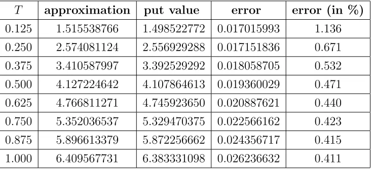
Example 3.11 In table 3.1 and fig. 3.1, we check the goodness of the approximation for a Hull and White model as a function of time to maturity. We can see that the performance
remains stable except for very smallT.
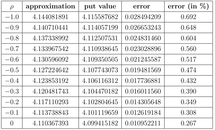
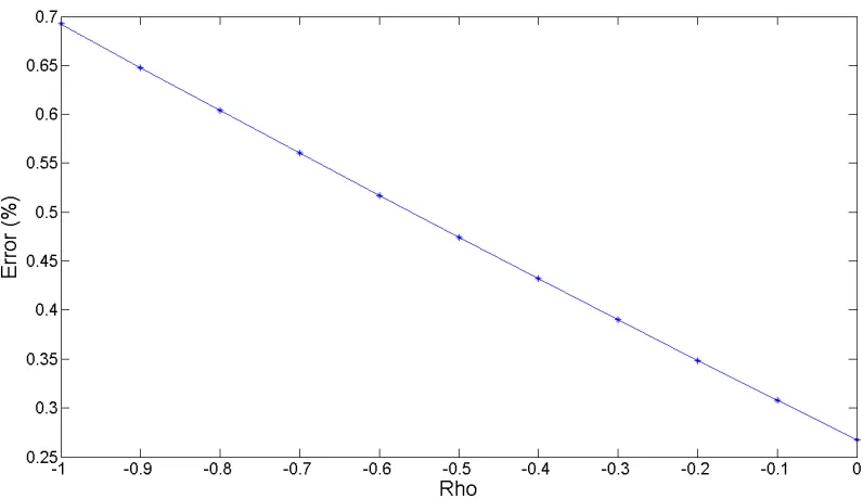
Example 3.12 In table 3.2 and fig. 3.2, we study the goodness of the approximation for a Hull and White model as a function of correlationρ. Observe that the relative error decreases
as the correlation goes to 0, as shown at the boundary.
Example 3.13 In fig. 3.3, we plot the goodness of the approximation for a Hull and White model as a function of the correlation ρ and the volatility of volatility γ. The relative error
[image:47.612.123.491.515.682.2]increases with increasing |ρ| and γ, agreeing with our approximation formula.
Table 3.1. Error of approximation as a function ofT in a Hull and White model. We take parameters S0 = 100, K = 97, r= 0.01, µ= 0.2,γ = 0.1, v0 = 0.04, ρ=−0.5.
Table 3.2. Error of approximation as a function ofρ in a Hull and White model. We take
S0 = 100,K = 97, r= 0.01, µ= 0.2, γ = 0.1, v0 = 0.04, T = 0.5.
ρ approximation put value error error (in %)
−1.0 4.144081891 4.115587682 0.028494209 0.692
−0.9 4.140710441 4.114057199 0.026653243 0.648
−0.8 4.137338992 4.112507531 0.024831460 0.604
−0.7 4.133967542 4.110938645 0.023028896 0.560
−0.6 4.130596092 4.109350505 0.021245587 0.517
−0.5 4.127224642 4.107743073 0.019481569 0.474
−0.4 4.123853192 4.106116312 0.017736881 0.432
−0.3 4.120481743 4.104470182 0.016011560 0.390
−0.2 4.117110293 4.102804645 0.014305648 0.349
[image:48.612.104.503.393.624.2]−0.1 4.113738843 4.101119659 0.012619184 0.308 0 4.110367393 4.099415182 0.010952211 0.267
Figure 3.2: Error of approximation as a function of correlationρin the Hull and White model whenS0 = 100, K = 97, r= 0.01, µ= 0.2,γ = 0.1,v0 = 0.04, T = 0.5.
[image:49.612.101.515.404.632.2]3.4.2
Stein & Stein model
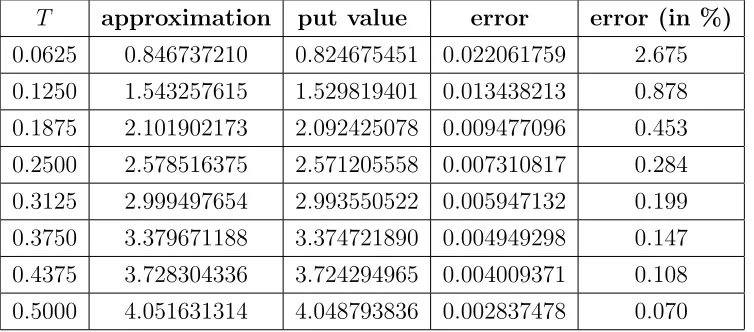
Example 3.14 In table 3.3 and Fig. 3.4, we check the goodness of the approximation for a Stein & Stein model as a function of time to maturity. We can see that the performance
remains stable except for very smallT.
Example 3.15 In table 3.4 and Fig. 3.5, we study the goodness of the approximation for a Stein & Stein model as a function of correlation ρ. Observe that the relative error decrease
as correlation ρ goes to 0, as shown in the boundary.
Example 3.16 In Fig. 3.6, we plot the goodness of the approximation for a Stein & Stein model as a function of correlation ρ and volatility of volatility γ.The relative error increases
[image:50.612.119.496.439.605.2]with the increasing of |ρ| and γ, agreeing with our approximation formula.
Table 3.3. Error of approximation as a function of T in the Stein & Stein model. We take
S0 = 100, K = 97, r = 0.01, κ= 4, θ = 0.2, γ = 0.1, v0 = 0.2,ρ=−0.5.
T approximation put value error error (in %)
Table 3.4. Error of approximation as a function of ρ in the Stein & Stein model. We take
S0 = 100, K = 97, r = 0.01, κ= 4, θ = 0.2, γ = 0.1, v0 = 0.2,T = 0.5.
ρ approximation put value error error (in %)
−1.0 4.098634963 4.093649507 0.004985456 0.122
−0.9 4.089234234 4.084699503 0.00453473 0.111
−0.8 4.079833504 4.075740491 0.004093013 0.100
−0.7 4.070432774 4.066771062 0.003661712 0.090
−0.6 4.061032044 4.057789459 0.003242585 0.080
−0.5 4.051631314 4.048793836 0.002837478 0.070
−0.4 4.042230584 4.039782435 0.002448149 0.061
−0.3 4.032829855 4.030753725 0.00207613 0.052
−0.2 4.023429125 4.021706504 0.001722621 0.043
[image:51.612.118.500.390.615.2]−0.1 4.014028395 4.012639987 0.001388408 0.035 0 4.004627665 4.003553874 0.001073791 0.027
Figure 3.6: Error of approximation as a function of correlation ρ and volatility of volatility
γ in the Stein & Stein model when S0 = 100, K = 97, r = 0.01, κ = 4, θ = 0.2, v0 = 0.2,
T = 0.5.
3.4.3
Heston model
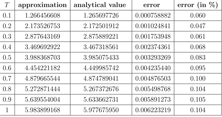
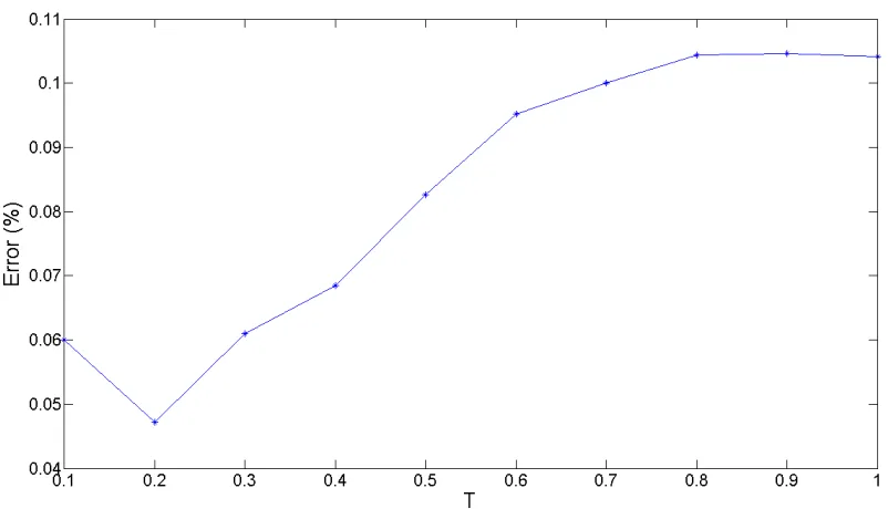
Example 3.17 In table 3.5 and fig. 3.7, we check the goodness of the approximation for a Heston model as a function of time to maturity. It is easy to see that our approximation
formula performs well, in particular for short time to maturity, and that the relative error
increases with T as to be expected.
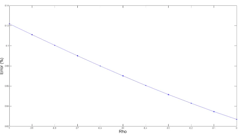
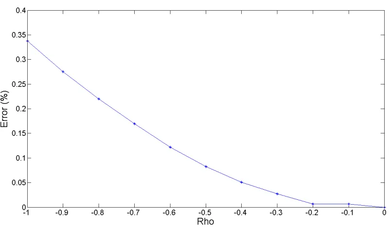
Example 3.18 In table 3.6 and fig. 3.8, we study the goodness of the approximation for a Heston model as a function of correlation ρ. The relative error decreases as the correlation ρ
goes to 0, as shown at the boundary.
Table 3.5. Error of approximation as a function of T in a Heston model. We take S0 = 100,
K = 97, r= 0.01, κ= 4, θ = 0.04, γ = 0.2,v0 = 0.04, ρ=−0.5.
T approximation analytical value error error (in %)