Essays on the skill premium and the skill bias of technological change

(1)

Essays on the Skill Premium and the Skill

Bias of Technological Change

Barbara Richter

A thesis submitted to the Department of Economics of the London

School of Economics for the degree of Doctor of Philosophy,

(2)

Declaration

I certify that the thesis I have presented for examination for the PhD degree of the

London School of Economics and Political Science is solely my own work other

than where I have clearly indicated that it is the work of others (in which case

the extent of any work carried out jointly by me and any other person is clearly

identified in it).

The copyright of this thesis rests with the author. Quotation from it is

permit-ted, provided that full acknowledgment is made. This thesis may not be

repro-duced without the prior written consent of the author.

I warrant that this authorization does not, to the best of my belief, infringe the

rights of any third party.

I declare that my thesis consists of about 40000 words.

Frankfurt, November 6, 2013

(3)

List of Tables

1.1 Main Parameter Specification . . . 34

1.2 Results for Different Values ofβandγ . . . 38

1.3 Simulation results for different values ofα . . . 43

1.4 Estimation results forα . . . 45

1.5 Preferred Parameter Specification, Part 2 . . . 51

1.6 Skilled Industries . . . 52

1.7 Unskilled Industries . . . 53

2.1 List of Industries Covered and the Main Parameters . . . 66

2.2 Growth Rate Differentials . . . 74

3.1 Descriptive Statistics . . . 98

3.2 Elasticities of Substitution . . . 107

3.3 Effect of Technological Progress on Input Use and Saving across Industries . . . 109

3.4 ICT Effect and Technology Bias . . . 111

3.5 Estimation Results . . . 118

3.6 Estimation Results (cont’d) . . . 119

3.7 Estimation Results (cont’d) . . . 120

(8)

List of Figures

1.1 Skilled Hours Worked . . . 30

1.2 Log Wage Premium . . . 31

1.3 Simulation Results on Growth Rates of Skilled and Unskilled La-bor Efficiency . . . 35

1.4 Simulation Results on Evolution of Skilled and Unskilled Capital per Hour Worked . . . 35

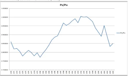
1.5 Relative Price . . . 46

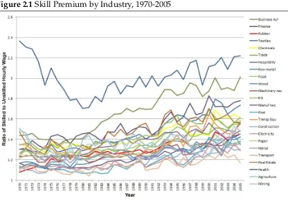
2.1 Skill Premium by Industry, 1970-2005 . . . 55

2.2 Share of Skilled Hours Worked by Industry, 1970-2005 . . . 56

2.3 Labor Share in Chemical Industry Over Time . . . 70

(9)

Acknowledgments

First and foremost, I am very grateful to my supervisor Francesco Caselli for

his considerable patience and constant support. I would like to thank my

ad-visor Rachel Ngai, Ethan Ilzetzki, Zsofia Barany, Nathan Converse, and Thomas

Schelkle for helpful discussions. Ashwini Natraj has been the most helpful

part-ner in debate, and I owe her many thanks. Further, I would like to thank my

colleagues at KfW for their moral support and understanding, and my parents,

my sister and her partner for their encouragement in difficult times. Last, but far

from least, I would like to thank my husband Johannes for six years of patience

and support.

Financial support from the ESRC and a LSE Research Scholarship is gratefully

(10)

Abstract

Using a two-sector model of production with potentially different capital shares

in each sector, I show that the evolution of the skill premium from 1970 to 2005

is consistent with skill-neutrality and even a mild unskill-bias of technological

change for plausible values of capital shares. The main channel of adjustment to

changes in labor supply is instead via the reallocation of capital. New investment

occurs predominantly in the skilled sector, to the detriment of the unskilled sector

of the economy. This result is shown both theoretically in a simple model and in

a quantitative exercise using data on the US economy.

Repeating the exercise with industry level data for the US reveals that there

has indeed been skill-biased technological change in a number of industries (such

as Business Activities and Health), while others have experienced skill neutral

and unskill-biased technological change (e.g. Agriculture). This difference in

results across industries is largely due to very different capital shares.

Finally, I look at the impact of the increasing importance of information and

communication technology (ICT) on the production function and the skill

pre-mium in each industry. I estimate a translog price function with skilled and

un-skilled labor, ICT capital and non-ICT capital as factors of production and find

that most industries exhibit ICT capital-skill complementarity. For most

indus-tries, technological progress has led to an increased use of both types of capital,

but the results on skill-biased technological change are as mixed as in chapter

two. ICT has affected the skill premium negatively in nearly two thirds of the

(11)

Introduction

The evolution of the skill premium in the US is a well documented fact. The

premium that a skilled worker can earn relative to an unskilled one has grown

by more than 20 % in the period from 1970 to 2005. At the same time, however,

the supply of skilled workers relative to unskilled workers has also increased,

making the rise in the skill premium a bit of a puzzle. Remarkably, the rise in

relative supply and relative wage has occurred in nearly all industries, though to

differing degrees.

The solution to this puzzle is often attributed to skill-biased technological

change (SBTC), technological progress that has enhanced the productivity of skilled

labor more than the productivity of unskilled labor. One possible manifestation

of this progress in technology is the rise in information and communication

tech-nologies (ICT).

In three essays, I check this solution to the puzzle against the data. First, I

simulate a fairly standard model of SBTC, but allow for an additional channel

of adjustment to changes in labor supply: the reallocation of capital investment

from the unskilled to the skilled sector. I find that there are plausible parameter

values for which this channel is strong enough to explain the evolution of the skill

premium without resorting to SBTC.

For the second essay, I look at twenty-two US industries separately. Ten of

these industries exhibit SBTC, twelve do not. Aggregating results to the sectoral

level, the primary sector clearly has not seen SBTC, whereas the manufacturing

(12)

across industries have not been uniform, but for the subsample from 1990

on-wards most of them have experienced some SBTC. As this is the period in which

ICT, in the form of computers, has come to be widely used, the next logical step

is to investigate the relationship between ICT and the skill premium.

Therefore, in the third essay, I estimate a translog production function,

sep-arately for each of twenty industries, to determine the role ICT capital plays in

the production function and in the evolution of the skill premium. I find that ICT

capital and skilled labor are complementary inputs in production for the

major-ity of industries. In most industries, technological progress has led to more use

of capital, both ICT and non-ICT, and to labor saving. The overall effect of ICT

capital on the skill premium is negative in fourteen of the twenty industries.

Taken together, my results suggest that the increase in the skill premium in

most industries and in the economy as a whole is only partly due to SBTC, if at

all. Shifts in capital investment, and mostly non-ICT capital investment at that,

(13)

Chapter 1

The Skill-Bias of Technological

Change and the Evolution of the

Skill Premium in the US Since 1970

1.1

Introduction

From 1970 to 2005, the premium that a college educated worker can earn

rela-tive to a worker without a college degree has risen by more than 20% in the US,

even though the relative supply of college educated labor has also increased

dur-ing that time. This is commonly attributed to skill-biased technological change

(SBTC). I show that this rise in the skill premium1could also be the result of cap-ital reallocation following the increase in the relative supply of skilled labor that

can be observed in the data. Technological change would be close to neutral in

that case, or biased towards the unskilled if anything.

Usually the line of reasoning to explain SBTC is as follows: the skill premium,

i.e. the relative price of college educated labor, has increased at the same time

as the relative supply of skilled labor. This is only possible if relative demand

for skilled labor has increased more than supply. The demand increase is then

1_{The terms “skill premium” and “college wage premium” are used interchangeably here. Both}

(14)

attributed to technological progress that favors skilled workers - i.e. SBTC.

By allowing for different capital shares in the skilled and unskilled sector

of production, I open up an additional channel through which the demand for

skilled labor can adjust to the observed increase in supply. If the initial level of

capital in the skilled sector is low and the capital share of the skilled sector is

higher than that of the unskilled sector, a large reallocation of capital is triggered

by the increase in the relative supply of skilled labor, leading to an increase in

pay-ment to skilled labor relative to unskilled labor.2 If the capital shares are different enough, it is even possible that there is so much capital reallocation that

techno-logical progress must favor unskilled workers to explain the skill premium.

This mechanism is, in brief, the driver behind the main result of this paper. I

simulate a two-sector model like the one in Caselli (1999), focusing on the effect

of an increase of the relative supply of skilled labor on the evolution of the skill

premium. The effects of changes to the skill premium on the decision to become

skilled are not considered here, nor is the origin of the increase in relative supply.

With this model I answer the following: Given the relative supply of skilled labor

observed in the data, how must skilled and unskilled capital and skilled and

unskilled production efficiency have evolved to yield the skill premium we see

in the data? I find that if the difference between skilled and unskilled capital

shares is large, unskilled production efficiency must have grown at least as fast

as skilled production efficiency for the model to be consistent with the wage and

skill supply data. This would suggest that there was no ongoing SBTC in the

period under study.

The analysis cannot capture one-off technology shocks that may have

oc-curred prior to 1970, however. Thus, if changes in the skill premium and the skill

supply since 1970 are consequences of a single technology shock before 1970 that

affects skilled production efficiency more than unskilled production efficiency,

the shock would not be picked up. The conclusion would still be that SBTC has

2_{Caselli (1999) points out that a fall in the wages of low-skilled workers, which also leads to}

(15)

played a small role at most in the changes to the skill premium.

That SBTC might not be the best explanation for the increase in the skill

pre-mium has been pointed out before, e.g. by Card and DiNardo (2002), who show

that SBTC fails along several dimensions of the distribution of wages. Beaudry

and Green (2002) show empirically that capital can play an important role. Still,

the majority of previous work attributes the increase in the skill premium to

SBTC. In empirical, mostly labor oriented, studies (e.g. Goldin and Katz (2007),

Autor, Katz, and Kearney (2008), among others, Katz and Autor (1999) provide

an overview), the change in labor demand is usually represented by a time trend

that does not distinguish between changes in technology and changes in the

allo-cation of capital. These shifts of labor demand can explain much of the evolution

of the skill premium. While the shifts are usually attributed to SBTC, it is equally

plausible to interpret them as an increase in skilled capital relative to unskilled

capital.

In theoretical models capital is included explicitly, but either differentiated

along a different dimension than “use by skill level” (e.g. equipment and

struc-tures as in Krusell, Ohanian, Rios-Rull, and Violante (2000) and Greenwood,

Her-cowitz, and Krusell (1997), among others) or assuming identical production

func-tions for all sectors (Caselli (1999), Galor and Moav (2000), Acemoglu (2002a), and

others). While the latter is a common assumption, it is not a priori certain that it

should hold in this case. The sectors of production in my model are

differenti-ated with regard to the skill level of the workforce. It is thus plausible to assume

that the capital and labor intensities are different in these sectors. Dropping the

assumption of equal capital shares across sectors can lead to very different

impli-cations with respect to SBTC.

There are other explanations for the evolution of the skill premium: it could be

due to a decrease in the minimum wage, which affects mostly low-skilled

work-ers and hence increases the premium (Fortin and Lemieux (1997), and more

(16)

in-creases the spread of wages paid (again, Fortin and Lemieux (1997), also

men-tioned in Gottschalk (1997)). One problem with the deunionization and

mini-mum wage explanations, though, is that the majority of the increase in the skill

premium is due to increases in wage inequality in the upper part of the wage

distribution (i.e. comparing the 90th wage decile to the 50th), while these

expla-nations mainly affect the lower end of the distribution (i.e. comparing the 50th

decile to the 10th; Acemoglu (2002b), Acemoglu and Autor (2010)). Barany (2011)

shows that a decrease in the minimum wage can have knock-on effects on the

upper part of the distribution, too, but the overall effect she finds is not large

enough to be the primary explanation.

Another possible explanation is an increase in trade openness, which leads

low-skilled production to move to other countries, reducing domestic demand

for low skilled workers (Johnson (1997), Topel (1997)). This explanation, while

appealing, cannot explain the timing of the increase (Acemoglu (2002b)) and the

overall effect is very small, as the US is not open enough to allow for a larger

effect.3 Burstein and Vogel (2010) find that international trade and multinational production together explain about 1/9thof the change in the skill premium.

Finally, the complementarity of skilled labor and capital (most famously

Krusell, Ohanian, Rios-Rull, and Violante (2000)) is given as an explanation.

While Krusell, Ohanian, Rios-Rull, and Violante (2000) claim it can account for

virtually all of the change in the skill premium, Ruiz-Arranz (2003) finds that

when allowing for the possibility of skill-biased technological change,

capital-skill complementarity explains at most 40% of these changes. While my results

show that skill-biased technological change is not necessarily present, doubts on

the importance of capital-skill complementarity remain.

3_{The relevant measure of openness here is the share of imports in total GDP. Production that}

(17)

Due to the assumption of different capital shares and the inclusion of an

irre-versibility constraint on capital investment, the model presented in section 1.2 is

too complex to allow the derivation of a closed form expression for the

equilib-rium path of skilled and unskilled capital. I will therefore show my main result

mathematically in a simplified version of the model in section 1.3 and then show

quantitatively that this result can also hold for the full model, even when

match-ing the model’s parameters to the US economy. Section 1.4 gives details of the

procedure and the derivation of these parameters, and the main results and

ro-bustness checks are presented in section 1.5. Section 1.6 concludes. Details on the

algorithm are relegated to the appendix.

1.2

The Model

1.2.1

Production Function

There are two types of production, skilled and unskilled, that are perfect

sub-stitutes in producing the final good. Each type of production is Cobb-Douglass.

Final output is given by:

Yt = As,tK_sβ_,_tL1_s_,−_t β+Au,tK_uγ_,_tL1_u−_,_tγ (1.2.1) where s and u denote variables pertaining to skilled and unskilled production respectively,Kis capital used in each type of production and Lis hours worked.

βis the skilled capital share, γ the unskilled one. A is a measure of production

efficiency4, and the relative growth rates of skilled and unskilled production ef-ficiency determine the bias of technological change. This model nests the case of

equal capital shares, but does not assume equality. In section 1.5 I look at the

con-sequences of relaxing the assumption of perfect substitutability between skilled

and unskilled production.

(18)

Skilled production today includes pharmaceuticals and telecommunications

equipment, where new production processes and very sensitive materials are

handled by highly skilled workers. Examples of unskilled production are the

textile and apparel industries, or food industries. Workers with college degrees

are unlikely to be found on the floor of a meatpacking plant.

The production function can be normalized to output per hour worked

yt = Yt

Lt

= As,tkβ_s_,_tϕ1_t−β+Au,tkγ_u_,_t(1−ϕt)1−γ (1.2.2) with ϕ ∈ (0, 1)the fraction of hours worked by skilled workers, for which there

is readily available data. In principle ϕ = 0 (only unskilled workers) and ϕ = 1

(only skilled workers) are possible, but as it is very unlikely that these extremes

ever occur in reality, I ignore them. Lower case letters are the per-hour-worked

equivalents to the elements of the final output production function.

1.2.2

Returns to Factors

The factors of production are paid their marginal products, so skilled wages are

ws,t = (1−β)As,tkβ_s_,_tϕ−_t β (1.2.3)

and the return to skilled capital is

rs,t =βAs,tk_sβ_,−_t 1ϕ1_t−β (1.2.4)

and similarly for unskilled wages and return to capital. The skill premium is

given by

ws,t

wu,t

= 1−β

1−γ As,t

Au,t

kβ_s_,_t kγ_u_,_t

ϕ−_t β

(1−ϕt)−γ (1.2.5)

Wages are increasing in both production efficiency and capital. An increase in the

(19)

asϕis increasing, too, which depresses the skill premium.

1.2.3

Irreversibility of Capital

The final good can be used for consumption or transformed into either type of

capital without cost. Once it has been transformed into one type of capital

how-ever, it cannot be changed into the other type, i.e. investment in either type of

capital is irreversible. Capital depreciates at a rate δj,j = s,u, that may or may not be the same for both types of capital. The constraints can thus be written as

k0_s ≥(1−δs)ksandk0u ≥(1−δu)ku.

There are two reasons for including this constraint: it strengthens the

cen-tral result of this paper, and it is realistic. The main mechanism I propose as

an alternative to skill biased technological change works via a shift of new

in-vestment from unskilled capital to skilled capital as a consequence of an increase

in the share of skilled hours worked. If the level of unskilled capital is higher

than is optimal, there can be no reallocation of the existing unskilled capital to

the skilled sector, only a reallocation of new investment. This slows down the

shift of capital to the skilled sector. As the increase in the skill premium requires

As,tkβs,t growing faster than Au,tkγu,t, this brake on the growth of skilled capital means that skilled production efficiency must have grown faster than it would if

there were no irreversibility constraint. Hence, the constraints bias the results

to-wards concluding that there has been SBTC. If the results show an unskill bias of

technological change nonetheless, this result is more robust as one important and

realistic obstruction to the adjustment channel I propose is already accounted for.

The realism of irreversible investment has been observed before. Bertola

(1998) notes that the market for used capital is thin or non-existent in most cases,

as the capital used for a certain type of production is of no value outside of this

production. As the two types of production in my model are very different, it is

plausible that the capital used in one type of production is of no value in the other

(20)

capital and vice versa. Caballero (1999) provides empirical evidence on

accumu-lation of capital that suggests the presence of an irreversibility constraint. In a

simulated RBC model, Coleman (1997) shows that introducing an irreversibility

constraint yields changes in the interest rate that better match the data than a

model without this constraint.

The constraint imposed is a very generic form of irreversibility, it simply

pro-vides a lower bound on the units of capital available in any given period. Similar

constraints have been used by Dixit (1995), Coleman (1997) and Bertola (1998).

There are other types of irreversibility, such as the vintage capital models used

by Jovanovic (1998) and Jovanovic and Yatsenko (2012), and the putty-clay

mod-els based on Johansen (1959). Both types assume that new investment can be

made in any type of capital, but once the investment is made, the installed capital

is fixed in the sense that there is no technological progress that could improve

existing capital. In vintage capital models, investment in new capital will always

be in the latest vintage. An additional feature of putty-clay models is that the

production function of each unit of installed capital becomes Leontieff, i.e. the

amount of labor that can work with each unit of this capital is fixed. Putty-clay

models were revived by Kehoe and Atkeson (1999) and Gilchrist and Williams

(2000), who find that these models yield better predictions of the behavior of

output and employment following a shock than the neoclassical model (without

irreversibility).

These ways of modeling irreversibility are not useful for the purposes of this

paper, however. As Bliss (1968) points out, technological progress in these models

is fully embedded in new capital. This is counterproductive when trying to

iso-late the path of technological progress from aggregate data. It is also not wholly

realistic, as innovation can take the form of an improvement of existing capital

(an easy example would be a free software upgrade). This could not be captured

via putty-clay and vintage models of capital. For the same reason, the

(21)

Innovations to existing capital can lead to changes in the units of labor required

(again, software upgrades are a useful example: an improved version of the same

software may mean work can now be done more efficiently by one person that

was previously done by two).

1.2.4

Households

There is a mass one of identical households, each with a measure one of members

who share all risks and income. Each household member inelastically provides

one unit of labor. Households’ per-period utility function is logarithmic and they

discount the future with factorρ. I check the robustness of my results to the choice

of utility function later on.

A share ϕt of members of each household is skilled each period. At the begin-ning of each period, unskilled members of the household can choose to become

skilled5, then production occurs, incomes are earned, and investment decisions for the following period are taken. Each investor decides on their investment

taking everyone else’s decision on investment and the relative supply of skills as

given.

The decision to become skilled or remain unskilled is not modeled explicitly,

as I am not interested in the reasons determining skill acquisition, but only need

to know the resulting relative skill supply. I can observe this relative skill supply

in the data. Any explicit model of skill acquisition decisions would need to match

this data and thus not affect the main results of this paper, therefore I simply use

the data directly and treat labor supply as given.

5_{Only unskilled household members take this decision, as an education generally cannot be}

(22)

1.2.5

Equilibrium

Households maximize lifetime utility subject to the resource constraint and the

irreversibility constraints on investment. The model is in discrete time, each unit

of time corresponding to a year.6

max{ks,t+1,ku,t+1}∞t=0U =

∞

∑

t=0

ρtln(ct) (1.2.6)

s.t. ct+ks,t+1+ku,t+1 ≤yt(ks,t,ku,t) + (1−δs)ks,t+ (1−δu)ku,t ∀t ≥0

kj,t+1 ≥(1−δj)kj,t ∀t ≥0, j∈ s,u

kj,t+1 >0 ∀t ≥ −1, j∈ s,u

ks,0,ku,0 given

Households know their future paths of labor supply and the evolution of

produc-tion efficiency, there is no uncertainty in the model.

In equilibrium, the following first order conditions must hold:

1

ct

+µj,t =ρ 1 ct+1

(1−δj+rj,t+1) +ρµj,t+1(1−δj) (1.2.7) where j =s,uandµj,t is the Lagrange multiplier on the irreversibility constraint for capital of type jat timet.

As long as the irreversibility constraint is not binding, the rates of return on

both types of capital are equal and determine consumption growth.

ct+1

ct

=ρ(rs,t+1−δs+1) =ρ(ru,t+1−δu+1) (1.2.8) Whenever the constraint becomes binding for one type of capital,

consump-tion growth is determined by the rate of return to that type of capital for which

the constraint is not binding.

(23)

1.2.6

Balanced Growth Path

Let ¯gbe the growth rate of output on the balanced growth path, and let ¯gsand ¯gu be the BGP growth rates of As andAu, respectively.

Proposition 1. If g¯ = ₁₋1

βg¯s =

1

1−γg¯u, 0 < ϕ < 1is constant and the irreversibility constraint is not binding, then there exists a Balanced Growth Path on which y, c, ksand

ku grow at constant rates.

Proof. The proof proceeds in three steps: first, I use the Euler equation to establish the relationship between the production efficiency and capital growth rates of

each type of production. Next, I derive the growth rate of total output and finally

I show that for the economy to be on the BGP the above equality has to hold.

Starting from the Euler equation

1+gc =ρ(βAskβ

−1

s ϕ1−β+1−δs) =ρ(γAukuγ−1(1−ϕ)1−γ+1−δu), (1.2.9) I look at the change in the growth rate of consumption gc from one period to the next, keeping in mind thatδs, δu, ρare constants, and that ϕis also constant on

the BGP:

1+g0c 1+gc

= βA

0

sk 0

β−1

s ϕ1−β+1−δs

βAskβs−1ϕ1−β+1−δs

= γA

0

uk 0

γ−1

u (1−ϕ)1−γ+1−δu

γAukγu−1(1−ϕ)1−γ+1−δu

(1.2.10)

BGP requires that 1+g0c

1+gc =1, so (1.2.10) leads to

βA0_sk

0 β−1

s ϕ1−β =βAskβs−1ϕ1−β (1.2.11)

and further to

1+gs = (1+gks)1−β. (1.2.12)

The same process yields

(24)

The growth rate of total output is simply

Y0

Y =1+g =

(1+gys)Ys+ (1+gyu)Yu

Ys+Yu . (1.2.14)

The growth rate of skilled output in turn is

1+gys = (1+gs)(1+gks)β =1+gks, (1.2.15)

making use of (1.2.12) in the second equality, and similarly for the growth rate of

unskilled output, making use of (1.2.13).

Next, using the fact that on the BGP 1₁+₊g_g0 = 1 together with (1.2.15) and the equivalent equation for unskilled output and capital, it can be shown that gks =

gku. Plugging this result back into (1.2.14) yields 1+g¯ = 1+gks = 1+gku. Using (1.2.12) and (1.2.13) and approximating by taking logs yields the conditions

stated.

Note that the condition is an approximation only in the discrete case. It holds

exactly in continuous time. This result, excepting the irreversibility constraint, is

also used in Caselli and Coleman (2001).

The condition of a constant share of skilled hours worked must always hold

on a balanced growth path. Ifϕwere growing at a constant rate on the balanced

growth path, as ϕ → 1, wu → ∞, providing an incentive for some individuals to remain unskilled and thus stopping the growth in skilled hours worked. This

would be inconsistent with a constant growth rate. For the same reason, ϕcannot

be growing at a negative constant rate on the balanced growth path.

As there will always be an incentive for someone to become skilled ifϕgoes to

zero and to remain unskilled ifϕapproaches one, the corner cases of only skilled

and only unskilled labor can only occur as a consequence of a discrete jump. Such

a jump is extremely unlikely to occur.

(25)

for example, ku would decrease at rateδu. This would raise the rate of return on

unskilled capital, ru. At some point, ru ≥ rs would be reached, at which point investment in ku is worthwhile again. Thus, a binding irreversibility constraint on investment in unskilled capital cannot be part of a balanced growth path.

Fol-lowing the same reasoning on ks leads to the conclusion that the irreversibility constraint cannot be binding for skilled capital on the balanced growth path

ei-ther. A binding irreversibility constraint on both types of capital at the same time

would lead to a decline in total capital and is equivalent to a binding

irreversibil-ity constraint in a one sector economy. Sargent (1980) and Olson (1989) show that

this is not possible on the BGP.

In order to assess local stability of the BGP consider, without loss of generality,

a one time shock toks. A negative shock will cause the level of skilled capital to fall below its BGP level. This leads to an increase of rs relative toru, leading to more investment in ks and thus a growth rate of skilled capital above the BGP growth rate. Eventually, the difference between the rates of return disappears

and the two types of capital grow at constant rates again. If there is a positive

shock, ks will rise above its BGP level. rs falls below ru and investment in ks slows or even ceases altogether if the irreversibility constraint becomes binding.

This will continue until the rates of return equalize and both types of capital grow

at constant rates again.

1.3

An Illustration of the Central Mechanism

To illustrate the channel through which a higher share of skilled labor can lead to

an increase in the skill premium, I use a simplified version of the model to show

the main result analytically: An increase in the skill premium can be consistent

with an increase in relative labor supply even absent any bias in technological

(26)

1.3.1

The Simplified Model

The economy is now a one period, two sector economy, with one sector skilled

and the other one unskilled. There is no irreversibility constraint and no

intertem-poral problem. An endowment of total capitalKis given exogenously, as are the levels of production efficiency. The only decision to be taken in this economy

is how to allocate this endowment of total capital between skilled and unskilled

capital.

Of particular interest is a comparative statics analysis of what happens to the

equilibrium skill premium when there is an infinitesimal change in the relative

supply of skilled labor, i.e. if ϕincreases.

1.3.2

The Main Result

Let k∗s

k be the initial equilibrium share of skilled capital in the economy.

Proposition 2. Iff β > γ and ϕ > k

∗

s(β,γ,ϕ,k)

k or β < γ and ϕ <

k∗s(β,γ,ϕ,k)

k , then d(ws

wu) d(ϕ) >0.

Proof. First, find the total differential of the skill premium with respect to skilled labor share. This differential will be greater than zero iff

(βk−_s 1+γk−_u1)dks dϕ >βϕ

−1₊

γ(1−ϕ)−1 (1.3.1)

Finding the total differential of skilled capital with respect to the skilled labor

share and plugging into the inequality above yields

β(1−γ)k−s 1(1−ϕ)−1+γ(1−β)k−u1ϕ−1 >β(1−γ)k−u1ϕ−1+γ(1−β)k−s 1(1−ϕ)−1. (1.3.2)

This can be simplified further to

(27)

which is true whenever the conditions stated in the proposition hold.

The first set of conditions states that it is possible to observe an increase in the

skill premium following an increase in the relative supply of skilled labor, if the

skilled sector is more capital intensive but its equilibrium share of capital is lower

than its share of labor. This suggests that the increase in the skill premium with an

increase in the relative supply of skilled labor is more likely if the skilled sector is

small initially, where the indicator of sector size is the share of capital in the sector

relative to total capital in the economy. As capital is used more intensively in the

skilled sector (which is what the first condition tells us), a lower level of capital

can produce a lot of output. When the availability of the other input increases,

however, it becomes desirable to substantially increase capital as well.

The second set of conditions reverses the inequality signs and the intuition

behind it: now, if the less capital intensive sector (the skilled sector now) sees an

increase in labor, the large share of skilled capital in total capital increases further.

This is because the more labor intensive sector now gets more of the production

factor it uses more intensively anyway, making it optimal to also give it more of

the less-intensively used factor.

Note that if β = γ, d

(ws

wu)

d(ϕ) > 0 is impossible. Assuming equal capital shares

ex ante thus automatically leads to the conclusion that skill demand must have

increased due to SBTC.

1.3.3

Relationship to Specific Factors Model

The simple model described here is a version of the specific factors model

well-known in the trade literature (see Jones (1971)). Here, the specific factors are

skilled and unskilled labor, and capital is the common factor.

Note that having β > γ means that production in the skilled sector is more

capital intensive than in the unskilled sector. One result for specific factor models

(28)

equilibrium. In my version this result means that an increase in the amount of

skilled labor leads to a more than one-for-one increase in skilled capital in

equi-librium, as each additional worker will be able to use capital more efficiently than

in the other sector, providing higher returns to the owner of capital. By analogous

reasoning, if the amount of unskilled labor decreases, this leads to a more than

one-for-one decrease in unskilled capital. If the initial equilibrium level of skilled

capital is low enough, the reallocation of capital will be so large as to overcome

the downward pressure on the skill premium due to the increase in skilled labor.

1.4

The Quantitative Exercise

The full dynamic model cannot be solved analytically. This section describes the

quantitative exercise, the data series used, and the choice of parameters.

1.4.1

The Idea

I perform a growth accounting exercise that allows me to back out the

unobserv-able paths of skilled and unskilled capital and skilled and unskilled production

efficiency from the observed paths of skilled and unskilled wages and skilled and

unskilled labor supply. Finding capital in this way is a departure from standard

growth accounting, where capital is taken from national accounts data. Here,

capital is determined endogenously for three reasons. First, while it is easy to

separate skilled and unskilled labor in the data, the distinction is much less clear

for capital. Is all capital used in a sector dominated by skilled labor automatically

skilled capital? Or only a constant fraction? What exactly is the difference

be-tween skilled and unskilled capital? Letting the model determine the allocation

of capital circumvents these issues. Second, capital data in the national accounts

is imperfectly adjusted for quality changes and hence technological progress.

Us-ing these data might lead to an understatement of the increase in production

(29)

assumption of reversible investment. This assumption is violated whenever the

irreversibility constraint on investment is binding for one type of capital.

Ignor-ing this violation introduces a bias into the sectoral capital data.7

The optimization problem in 2.6 can be solved either by Lagrangian or by

value function iteration. The former is more useful in illustrating the formal

equi-librium and hence was used in section two. Value function iteration on the other

hand is easier to implement quantitatively, especially when dealing with the

ad-ditional irreversibility constraints on investment. The results are the same using

either method.

The exercise starts with an initial guess on a sequence for As and Au. With this guess I can recursively solve

V(ks,ku,As,Au) =max k0s,k0u

ln(c) +ρV0(k0s,k0u,A0s,A0u) (1.4.1)

s.t. k0_s ≥(1−δs)ks, k0u ≥(1−δu)ku

with c = y(ks,ku,As,Au,ϕ) + (1−δs)ks + (1−δu)ku −k0s−k0u, and ϕas taken from the data as described below. This yields optimal paths forks and ku which are then combined with the sequences for As and Au guessed previously and ϕ

as taken from the data to derive the wage sequencesws and wu that are implied by the model. These sequences of wages are then compared to the actual wage

data. If the sum of squared differences between the wages in the model and in

the data is above a critical value, the sequences of ks and ku and the data on wages and ϕ are used to update the guess for As and Au via As = wsϕ

β

(1−β)ks and

Au = wu(1−ϕ)

γ

(1−γ)ku . With this new guess, the value function iteration starts over. This process is repeated until the sum of squared differences between

model-generated wages and wage data falls below the critical value.

In order to run this exercise, I need data series forϕ,wsandwu, and parameter

7_{More specifically, this bias is introduced through the aggregation weights. One assumption in}

(30)

values for β, γ, δs, δu, and ρ. Their derivation is described in the next section.

More detail on the algorithm can be found in the appendix.

1.4.2

The Data

The data used in this paper is either directly taken or derived from the EU KLEMS

dataset (EUKLEMS (2008), also see Timmer, O’Mahony, and van Ark (2007)) on

the US economy. The dataset builds on Jorgenson, Ho, and Stiroh (2003)’s work

in growth accounting and collects data on, among other things, wages, different

types of capital and output by industry.8

1.4.2.1 Labor Supply and Wages: ϕ,ws, andwu

Labor market data by skill is available in three categories in the dataset:

high-skilled (college graduate and above), medium-high-skilled (high school graduate and

some college) and low-skilled (did not complete high school). As the model

re-quires two types of skill, one third of the medium-skilled values in labor

compen-sation and hours worked data are added to the corresponding high-skill values to

yield theskilledvariables and two-thirds of the medium-skilled values are added to the low-skill values to deliverunskilledvariables. This is to reflect the fact that someone who dropped out of college just before graduation will have

consider-ably more education than someone who left after the first term, even though both

are classified as medium-skilled. Using one third and two thirds to separate them

yields a skill premium that is close to what others have found.

The share of skilled hours worked ϕis simply hours worked by skilled

work-ers divided by hours worked by all workwork-ers, and similarly for unskilled labor.

8_{Most empirical studies of the skill premium use data from the Current Population Survey}

(31)

[image:31.595.114.541.99.362.2]

Figure 1.1Comparing the Share of Skilled Hours Worked from EU KLEMS Data and from Autor, Katz, and Kearney (2008)

Skilled hourly wages are derived by multiplying the skilled workers’ share in

la-bor compensation with total lala-bor compensation and dividing the total by skilled

hours worked (share of skilled hours worked times total hours worked).9 The analogous procedure is used for unskilled hourly wages.

Figure 1.1 compares the share of skilled hours worked according to my

deriva-tion and using the data from Autor, Katz, and Kearney (2008). The series move

in parallel, and Autor, Katz, and Kearney (2008)’s share of skilled hours worked

is slightly lower throughout. As a robustness check I run the simulation with the

Autor, Katz, and Kearney (2008) values and find that there is virtually no

differ-ence in the results.

Figure 1.2 shows the log of the skill premium my procedure yields and

com-pares it to the log of the skill premium used in Autor, Katz, and Kearney (2008),

both normalized to one in 1970. Similarly to the skill share in hours, my data

se-ries is below Autor, Katz, and Kearney (2008)’s sese-ries, and they move in parallel

9_{The data series by name and formulas used are: H HS+1/3 H MS for high skilled hours}

(32)

[image:32.595.113.543.91.360.2]

Figure 1.2 Comparing the Log Wage Premium from EU KLEMS Data and from Autor, Katz, and Kearney (2008)

for most of the period under consideration.

Labor compensation may also include non-wage payments to the worker and

other benefits, so it is not a perfect measure from which to derive wages. This

may go some way towards explaining the remaining difference from Autor, Katz,

and Kearney (2008)’s series. Eckstein and Nagypal (2004) find however that

la-bor compensation data and wage data move largely parallel. In any case, as the

present study is an accounting exercise at heart, total labor compensation is the

more appropriate measure.

1.4.2.2 Initial Values for Skilled and Unskilled Capital and the Production Efficiencies

The initial levels of skilled and unskilled production efficiencies are normalized

to one. In order to find model-consistent initial values I have to either assume

equal production efficiencies in the first period or equal rates of return on

(33)

restrictive10.

To start the iteration, I need to specify a first guess for the full sequence of

skilled and unskilled production efficiency. The initial guess sets the first period’s

skilled and unskilled production efficiency equal to one. For all further periods

it is simply assumed that both types of production become more efficient at the

same constant rate, the long run growth rate.

The initial values for skilled and unskilled capital are obtained from the

equa-tions for the skilled and unskilled wage respectively. The values for capital

are the only unknowns in the wage equations ws,0 = (1−β)As,0kβs,0ϕ

−β

0 and

wu,0 = (1−γ)Au,0kγ_u_,0(1−ϕ0)−γ, soks,0 andku,0 can be found by simply solving

for them.

1.4.2.3 Capital Shares: βandγ

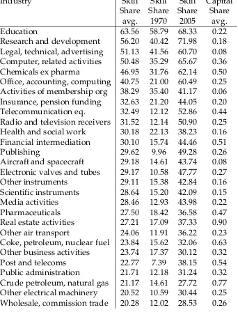
As the model has two sectors, skilled and unskilled, I classify the industries in

the dataset into skilled and unskilled. To that end, I rank all industries at the

highest-digit level for which data are available11 by the average of the share of high-skilled (in the three-skill-level definition) hours worked in 1970 and 2005.

Over the period studied, the share of high-skilled labor has increased in all

in-dustries, sometimes substantially. This trend has been observed first by Berman,

Bound, and Griliches (1994) for manufacturing industries from 1979 to 1989.

Au-tor, Levy, and Murnane (2003) and Spitz-Oener (2006) (for Germany) show that

this trend is not due to a change in the type of jobs available, but to an increase

in skill requirements for the same job. They attribute the increased skill

require-ments to SBTC. As this increase has been observed across all industries, the fact

that it might be due to SBTC should not bias my results. One further indication

that this method of finding capital shares should not introduce a bias is that using

10_{Assuming equal rates of return in the first period results in skill neutral to unskill-biased}

technological change for a wider range of values for the capital shares. Normalizing production efficiencies thus also is the more conservative assumption.

11_{If I only have data for the one-digit industry, I use that; if there is data for three-digit industries}

(34)

either the 1970 high-skill shares or the 2005 shares would not change the ranking

substantially.

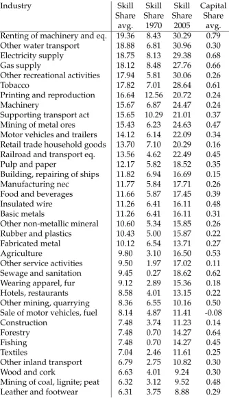
All industries with an average share of hours worked by high-skilled labor

of 20% or higher are considered part of the ”skilled” sector, the rest forms the

”unskilled” sector. Appendix 3 shows the industries’ ranking and their average

high-skill share of labor, along with the 1970 and 2005 shares. The cutoff of 20%

ensures that there are roughly the same number of industries in the skilled and

unskilled sector.

I start by calculating the labor share, i.e. the ratio of labor compensation and

value added in a sector (1−βi = LABVAii), for each industry every five years. Then I take the unweighted average of each industry over time (also given in Appendix

3) and then the average over all industries classified as skilled or unskilled

respec-tively, weighted by their average value added. The skilled and unskilled capital

shares are then derived as one minus the labor shares.

The resulting capital shares are β = 0.39 for skilled production andγ =0.29

for unskilled production, meaning the skilled sector is more capital intensive than

the unskilled sector. As the values for the capital shares are sensitive to the

defi-nition of sectors and the cutoffs chosen, I check the robustness of the simulation

results to different values ofβandγ.

1.4.2.4 Depreciation Rates: δs andδu

EU KLEMS breaks down the data on capital stock into eight types of capital: In-formation Technology, Software, Communication Technology, Transport Capital, Other Machinery,Other Construction,Residential Structures, andOther Capital. Each type of capital has its own depreciation rate that is constant across industries.

Differ-ences in depreciation rates between industries thus arise from differDiffer-ences in the

composition of their capital stocks. To find each industry’s depreciation rates at

one point in time, I take the average of the different depreciation rates, weighted

(35)

As capital stock data are not available at the same level of detail as labor and

output data, the level of capital stocks must be imputed for some industries. In

these cases, I assume that a three-digit industry’s share of capital in the one

digit-capital stock is the same as the three-digit industry’s share in value added.

Once I have each industry’s depreciation rate for every five years, I follow the

same sector division and averaging procedure as for capital shares. The resulting

depreciation rates are δs = 0.091 for skilled capital and δu = 0.079 for unskilled capital.

1.5

Quantitative Results and Robustness Checks

1.5.1

Main Results

The main parameter specification uses the values derived in section 1.4.2 and

pre-sented in table 1.1. The long run growth rate, which is needed for the algorithm, is

set tog =0.025 to correspond to the historic average US growth rate. The results are not sensitive to this choice, however. Some more technical parameters need

to be specified for the algorithm. These are given in table 1.5 in the appendix. The

robustness of results to different parameter specifications will be discussed later.

The simulation results for production efficiency growth and capital are shown

in Figures 1.3 and 1.4 respectively. Both production efficiency growth rates are

very high until about 1980 and considerably lower after that, consistent with the

productivity slowdown observed by others (see for example Nordhaus (2005)).

Until 1980 the growth rate for unskilled production efficiency is above the one for

skilled production efficiency, after 1980 the growth rates are much closer. Skilled

production efficiency grows 0.27 percentage points slower on average than

un-Table 1.1: Main Parameter Specification

Parameter β γ δs δu ρ

(36)

[image:36.595.110.541.120.392.2]

Figure 1.3 Simulation Results on Growth Rates of Skilled and Unskilled Labor Efficiency

[image:36.595.120.542.487.741.2]

(37)

skilled production efficiency, though the difference is 0.53 percentage points in

the first fifteen years and only 0.04 percentage points after 1985.

SBTC is said to be present if the growth of relative skilled production

effi-ciency leads to an increase in the relative marginal product of skilled labor (see,

eg, Caselli and Coleman (2001)), in which case the skill premium is increasing in As

Au. For this ratio to increase, skilled production efficiency needs to grow faster than unskilled production efficiency. The higher growth rate for unskilled

pro-duction efficiency here suggests then that there is unskill-biased technological

change if anything, though given the differences are small throughout,

consider-ing technological change as skill-neutral is more appropriate. This result can be

attributed to the combination of different capital shares in the two sectors and

very low initial levels of skilled capital. Part of the difference pre- and

post-1985 stems from a period between 1974 and 1982 in which the skill premium was

actually decreasing. In that time period, higher unskilled production efficiency

growth would be predicted by most models.

Both types of capital increase over the 35 years under consideration. Skilled

capital stays roughly constant in the early 1970s, grows very rapidly in the early

1980s and continues growing at a slightly lower rate. The average growth rate

for skilled capital is 8.84%. Unskilled capital decreases for the first few years

as the irreversibility constraint is binding. After that, unskilled capital grows

consistently. Overall, the average yearly growth rate for unskilled capital is 5.6%.

The reasons for slow capital growth in the 1970s can only be speculated on. It

could simply be a consequence of low economic growth following the oil shocks.

I could also be due to the 1970s being the early period of a new general purpose

technology (GPT, see, e.g. Aghion, Howitt, and Violante (2002)). This nascent

technology could have led to deferred investment, to be able to take advantage

of the new technology once it is better developed.

These results illustrate the additional adjustment mechanism present in the

(38)

unskilled to skilled capital. The magnitude of this shift depends on the relative

size of the capital shares in the two sectors.

1.5.2

Robustness Checks

The skill premium can be explained in absence of SBTC for plausible values of

the capital shares. This is need not be true universally, however. The overarching

question in this section is: If the wages and skill supply observed in the data were

generated by an economy not governed by the parameters used in section 1.5.1,

but by different ones, would the implications of these other parameters for SBTC

be the same? A number of robustness checks in this section show how the values

of capital shares matter, while other parameters are less important.

1.5.2.1 Different Capital Shares

There are two margins along which different capital shares might have an impact:

changes to the levels of β and γ and changes to the difference between the two

capital shares.

Table 1.2 provides a summary of the results using a wide array of values for

β and γ. The first two columns give the values for capital shares in the skilled

and unskilled sector and the third gives the difference between the two capital

shares. The fourth column shows the average difference between the skilled and

unskilled production efficiency growth rates over the whole sample period, and

the last two columns give the average difference for the two sub-periods from

1970−1985 and 1985−2005. The first row shows the values for the preferred

specification discussed in the previous section.

Looking at the difference in growth rates for the whole period, two

observa-tions are striking. First, SBTC is observed for β−γ ≤ 0.08, and the skill bias is

larger the smaller the difference between the capital shares. Second, the degree

of skill-bias is decreasing in the skilled capital share, even holding the difference

(39)

[image:39.595.176.475.93.375.2]

Table 1.2: Results for Different Values ofβandγ β γ β−γ gs−gu gs−gu gs−gu

1970-2005 1970-1985 1985-2005

0.39 0.29 0.1 -0.0027 -0.0053 -0.0004

0.42 0.32 0.1 -0.0035 -0.0069 -0.007

0.36 0.26 0.1 -0.0018 -0.0039 -0.0001

0.44 0.32 0.12 -0.0066 -0.0121 -0.0021

0.40 0.28 0.12 -0.0055 -0.0099 -0.0017

0.39 0.30 0.09 -0.0014 -0.0032 0.0002

0.38 0.29 0.09 -0.0011 -0.0028 0.0003

0.39 0.31 0.08 -0.0001 -0.0011 0.0008

0.38 0.30 0.08 0.0001 -0.0008 0.0009

0.37 0.31 0.06 0.0030 0.0040 0.0022

0.42 0.38 0.04 0.0046 0.0065 0.0030

0.40 0.36 0.04 0.0050 0.0072 0.0031

0.38 0.34 0.04 0.0054 0.0079 0.0033

0.36 0.32 0.04 0.0059 0.0087 0.0035

0.34 0.34 0 0.0014 0.0177 0.0061

0.32 0.36 -0.04 0.0169 0.0267 0.0087

0.29 0.39 -0.1 0.0252 0.0401 0.0127

capital shares determines the direction of the bias, the level of β the degree, as

can be seen from looking at the results forβ−γ=0.1 andβ−γ=0.04 with

dif-ferent values forβ. The positive value for the growth rate differential forβ=0.29

and γ = 0.39 shows that the results are not symmetric in the capital shares. The

turning point is atβ−γ =0.08, where the bias is very close to zero.

The results differ markedly across the two sub-periods under consideration

as well. The difference in growth rates is consistently closer to zero in the

sec-ond part of the sample. This is a bit puzzling in some cases, as the decline in the

skill premium in the early part of the sample would suggest a stronger unskilled

production efficiency growth rate and thus a narrowing of the difference. Two

possible explanations come to mind. The first is that the capital investment

chan-nel works in the opposite direction there, too, and the second that these values

for the capital shares are less likely to be correct.

The presence and degree of SBTC thus depends both on the level of the capital

shares and the difference between them: the higherβand the larger the difference

(40)

ad-ditional mechanism I propose, as the degree of capital reallocation will be larger

for larger differences between the capital shares. As the previous sections have

shown, values for which SBTC plays no role can be derived plausibly.

1.5.2.2 Different Depreciation Rates

For my main specification, the depreciation rates for the two types of capital are

different. It is possible that the initially binding constraint is due to this

differ-ence, and it is likewise possible that the higher production efficiency growth rate

in the unskilled sector is due to the irreversibility constraint being binding early

on. I therefore check how results change when the depreciation rates are equal

in both sectors. Ex ante I would expect largely the same result as before. The

main channel from which my result derives is the reallocation of capital

invest-ment, with different depreciation rates and the irreversibility constraint as

possi-ble blockages of this channel. Including these blockages in the model strengthens

the main result, as two important potential obstructions are already accounted

for. As the blockages do not narrow the main channel enough to qualitatively

affect the results, removing either one or both of them should not alter the main

result, though the precise values might be different.

This turns out to be true, as the production efficiency growth rates with equal

depreciations rates track the ones from my preferred specification. Only in the

earlier years is the skilled growth rate larger than in the main specification. This

is true whether I assume that both depreciation rates are equal to the skilled rate

or the unskilled rate, the results are nearly identical (−0.0032 for the higher rate,

−0.0033 for the lower one).

I also check results for a larger difference between the depreciation rates (δs = 0.12 compared to δu = 0.06) to see if results are sensitive to an understatement of the difference in depreciation rates. The growth rate differential in this case

is −0.0002, suggesting that a very large difference in depreciation rates might

(41)

Finally, I also consider much smaller depreciation rates, δs = 0.039 and

δu = 0.033. These are the values of the skilled and unskilled depreciation rates as calculated for 1970. The depreciation rates are increasing over time, as they

form the weighted average of the depreciation rates of skilled and unskilled

cap-ital used at each period. Over time, the types of capcap-ital with higher depreciation

rates increase, which leads to an overstatement of the depreciation rate for the

early periods. This matters, as depreciation rates determine the irreversibility

constraint, which is binding for several periods early on in the baseline scenario.

With these lower depreciation rates, I can test whether the binding constraint is

an artifact of taking the average depreciation rate. It turns out that with the lower

rates, the irreversibility constraint binds for one period only. The difference in

the growth rate of skilled and unskilled labor efficiency stays negative (−0.0039).

The main results are not affected.

1.5.2.3 Equal Depreciation Rates and Capital Shares

A further check is whether the results change if I assume equal capital shares and

equal depreciation rates in both sectors. This is the standard assumption in the

SBTC literature, and I would therefore expect the same result as in that literature,

namely that skilled production efficiency grows faster than unskilled production

efficiency.

In this case, with β = γ = 0.34, skilled production efficiency indeed grows

faster than unskilled production efficiency on average, with a difference of 1.07

percentage points. This indicates that with the assumption of equal capital shares

intact, the conclusion that SBTC drove the increase in the skill premium is valid.

1.5.2.4 Leaving Out the Irreversibility Constraint

Ignoring the irreversibility constraint should lead to a faster decrease in unskilled

capital and hence to a higher growth rate for unskilled production efficiency. This

(42)

As this has knock-on effect on skilled capital, the overall result changes little. The

growth rate of unskilled production efficiency is larger than the skilled growth

rate, with a difference of 0.0027.

1.5.2.5 Alternative Utility Function

So far, I have assumed that individuals have logarithmic utility, mostly because I

am interested in the capital reallocation process between sectors and less in

peo-ple’s overall investment decision. Log utility is convenient, as changes in the

interest rate do not affect the consumption allocation over time.

As consumption allocation, via the budget constraint, has effects on

invest-ment decisions, it is prudent to check that the results do not depend on the choice

of utility function. Therefore, I also look at the results from using a CRRA utility

function u(c) = c1₁−₋η−_η1, withη =2. On average, unskilled production efficiency

grows faster by 0.1 percentage points. The difference here is smaller in value, but

points in the same direction.

1.5.2.6 Alternative Data Derivation

I also test a different way of constructing the data for skilled and unskilled wages

and shares in hours worked. Choosing as a cutoff at least 30% highly skilled

workers in 2005 yields a wage premium and total skilled labor with the same

movements as in the data used above, but with slightly different absolute values.

This time, I take the initial values for skilled and unskilled capital directly from

the data. The caveats as to the appropriateness of the capital data remain.

In this version of data derivation, I leave out Real Estate Activities. It would classify as skilled given the cutoff I use, but is the sector with the largest change

in labor composition. To avoid the results swinging on the choice I make for this

sector, I prefer to leave it out altogether.

The capital shares in this case are slightly different: β = 0.3 and γ = 0.29,

(43)

re-sults remain the same: skilled capital increases fourfold, unskilled capital does

not quite double and skilled production efficiency grows slower than unskilled

production efficiency in more than half the periods. The average difference in

the growth rates is very small with unskilled production efficiency growing 0.3

percentage points faster.

1.5.2.7 A Different Production Function

The assumption of perfect substitutability of both types of production is fairly

restrictive, and it is not a priori obvious why it is a reasonable assumption to

make. Indeed, generalizing the production function to a CES function would

open another channel of adjustment to changes in labor supply via the change in

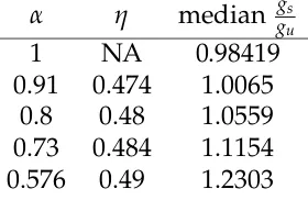
the relative price of the two kinds of output.

A more general production function would be

Y = [η(Askβsϕ1−β)α+ (1−η)(Aukγu(1−ϕ)1−γ)α] 1

α (1.5.1)

where σ = ₁₋1_α is the elasticity of substitution between skilled and unskilled

production and α ∈ (−∞, 1). Setting α = 1 yields the perfect substitutability

case.

The relative growth rate of labor efficiencies then is

gs

gu

= g

−β

ks

g−_kuγ(

ws,t+1/wu,t+1

ws,t/wu,t

)1α(ϕt+1 ϕt

)1α−1+β(1

−ϕt+1

1−ϕt

)1−1α−γ. (1.5.2)

It is decreasing in the absolute value of α. Skilled production efficiency grows

faster relative to unskilled production efficiency the poorer the substitutability

between the two sectors of production: With decreasing α the weight given to

growth in the wage premium and growth in relative labor supply increases,

whereas the weight given to the relative capital growth rates stays the same.

(44)

[image:44.595.255.395.95.186.2]

Table 1.3: Simulation results for different values ofα

α η median _ggs_u

1 NA 0.98419

0.91 0.474 1.0065

0.8 0.48 1.0559

0.73 0.484 1.1154

0.576 0.49 1.2303

to the growth rate of unskilled production efficiency. Changing α changes the

capital growth rates, too, as lowerαleads to higher growth rates of skilled capital

relative to unskilled capital, but this effect seems to not be strong enough to ke

Essays on the skill premium and the skill bias of technological change