Essays in macroeconomic theory: informational frictions, market microstructure and fat tailed shocks

(1)

Essays in macroeconomic theory:

informational frictions, market

microstructure and fat-tailed shocks

by

Marco Antonio Ortiz Sosa

A thesis submitted to the Department of Economics for the degree of

Doctor of Philosophy

at the

LONDON SCHOOL OF ECONOMICS

(2)

Declaration

I certify that the thesis I have presented for examination for the PhD degree of the London School of Economics and Political Science is solely my own work other than where I have clearly indicated that it is the work of others (in which case the extent of any work carried out jointly by me and any other person is clearly identified in it).

The copyright of this thesis rests with the author. Quotation from it is permitted, provided that full acknowledgement is made. This thesis may not be reproduced without the prior written consent of the author.

I warrant that this authorization does not, to the best of my belief, infringe the rights of any third party.

I declare that my thesis consists of approximately 54,000 words.

(3)

Statement of conjoint work

Chapter 1 of this thesis is based on research that I undertook while working as a Research Specialist at the Central Reserve Bank of Peru. This work was jointly co-authored with Dr. Carlos Montoro and I contributed a minimum of 50% of the work.

(4)

Abstract

This thesis is composed by five chapters. Chapter 1 presents a new Keynesian open economy model that includes risk-adverse foreign-exchange market dealers and foreign exchange intervention by the monetary authority. In this setup portfolio decisions made by dealers add an endogenous time variant risk-premium element to the traditional UIP that depends on FX intervention by the central bank and FX orders by foreign investors. We use the model to analyse the interactions between monetary policy and FX interventions.

Chapter 2 introduces information heterogeneity into the model presented in Chapter 1. As in Bacchetta and van Wincoop (2006), the “rational confusion” generated by the introduction of heterogeneous information magnifies the impact of the unobservable

capital flows shocks on the exchange rate.

Chapter 3 introduces fat-tailed shocks in the model of Kato and Nishiyama (2005). This is a simple new Keynesian model where the central bank explicitly considers the zero lower-bound constraint on interest rates. We find that shocks with ‘excess kurtosis’ make monetary policy relatively more aggressive far away from the zero lower bound region though, this difference reverts when the economy is close to this constraint. Under our baseline calibration, the difference between optimal policies under Gaussian and fat-tailed shocks is not quantitatively significant.

Chapter 4 presents a model in which investors form their expectations in an adaptive way to price bonds, in the spirit of Adam, Marcet and Nicolini (2011). We follow different assumptions regarding the learning process followed by agents. In the case of finite maturity bonds, the knowledge of the pricing of the first maturity will act as an ’anchor, limiting the price volatility of bonds with short maturities. As the maturity increases,

(5)

the price volatility converges to the one of the consol bond.

(6)

Acknowledgements

I would like to express my gratitude to all the people that contributed to this thesis.

First and foremost I am grateful to my supervisor, Wouter Den Haan, whose support has been invaluable. I am also grateful to my previous supervisors, Albert Marcet and Kosuke Aoki, who guided me through in the early stages of my research projects.

I am also grateful to those who contributed with this work either by reading and commenting on earlier versions of my chapters or by discussing specific aspects of them during my presentations at seminars and conferences, especially Carlos Montoro, Paul Castillo, Paolo Vitale, Stephen Cecchetti, Ramon Moreno, Hugo Vega and Philippe Bacchetta. I am also indebted to Julio Velarde, Vicente Tuesta, Marco Vega and Diego Winkelried for very fruitful discussions that led me to pursue this line of research.

I acknowledge financial support from the Central Reserve Bank of Peru.

Finally, I dedicate this thesis to my family, who have always given me their uncon-ditional support. In specific to my mother Dina, my father Gaspar, my uncle Miguel, my aunt Hilda, my grandma Hilda and my siblings Javier and Diana.

(7)

List of Tables

1.1 Baseline Calibration . . . 34

1.2 Macroeconomic volatility under FX Intervention Rules (No in-tervention ≡1) . . . 38

1.3 Macroeconomic volatility (No intervention ≡ 1), Low elasticity of subs. btw. home and foreign goods (ε= 0.4.) . . . 53

1.4 Macroeconomic Volatility (No intervention ≡1), High elasticity of subs. btw. home and foreign goods (ε= 1.5.) . . . 54

1.5 Macroeconomic volatility (No intervention ≡ 1), Low elasticity of subs. btw. exports and foreign goods (εF = 0.4.) . . . 55

1.6 Macroeconomic volatility (No intervention ≡1), High elasticity of subs. btw. exports and foreign goods (εF = 1.5.) . . . 56

1.7 Macroeconomic volatility (No intervention ≡ 1), Low domestic good price rigidity (θH = 0.25.) . . . 57

1.8 Macroeconomic volatility (No intervention ≡1), High domestic good price rigidity (θH = 0.95.) . . . 58

3.2 Robustness to alternative parameterisations . . . 119

4.1 Baseline Calibration: Case I . . . 136

4.2 Baseline Calibration: Case II . . . 136

5.1 Fisher equation model - maximum likelihood estimation . . . 158

5.2 Learning models - results of simulations . . . 181

(11)

List of Figures

1-1 Intervention in the foreign exchange market: 2009 - 20121 _{. . . .} ₁₅

1-2 Existence of equilibria under FX intervention rules . . . 37

1-3 Reaction to a 1% portfolio shock - ∆st rule. . . 40

1-4 Reaction to a 1% foreign interest rate shock - ∆st rule. . . 41

1-5 Reaction to a 1% foreign inflation rate shock - ∆st rule. . . 42

1-6 Variance decomposition of the exchange rate changes (∆st) . . . 43

1-7 Reaction to a 1% FX intervention shock - RER rule. . . 49

1-8 Reaction to a 1% portfolio shock - RER rule . . . 50

1-9 Reaction to a 1% foreign interest rate shock - RER rule. . . 51

1-10 Reaction to a 1% foreign inflation rate shock -RER rule. . . 52

2-1 Existence of equilibria under FX intervention rules (HI) . . . 75

2-2 Magnification effect for different values of σω∗ and σ_ν . . . 77

2-3 Reaction to unobservable and fundamental shocks under Heterogeneous Information and Common Knowledge . . . 79

2-4 Regression of ∆son unobservable and fundamental shocks - ∆srule . . . 80

2-5 Existence of equilibria under FX intervention rules (CK) . . . 85

3-1 Exponential Power family of distributions . . . 109

3-2 Value Function with Zero Lower Bound (baseline calibration) . . . 112

3-3 Optimal Policy Reaction Function (baseline calibration) . . . 113

3-4 Optimal reaction and Taylor rule under Gaussian and Laplace Shocks . . 114

3-5 Central Bank’s loss function, (Laplace - Gaussian) . . . 115

3-6 Distribution of shocks and the ZLB . . . 116

(12)

4-1 Case I: Std. Dev. of price/coupon ratio . . . 138

4-2 Case I: Evolution of beliefs . . . 139

4-3 Case II: Standard deviation of bond prices under learning . . . 140

4-4 Case II: Evolution of beliefs . . . 141

4-5 Case II: Yield volatility under learning . . . 143

4-6 Case II: Sensitivity to gain parameter . . . 143

5-1 Yields reaction to transitory and permanent shocks to inflation . . . 159

5-2 U.S. nominal yield curve . . . 161

5-3 UK 2.5% consol bond price (nominal, expressed in GBP£) . . . 179

(13)

Chapter 1

Foreign exchange intervention and

monetary policy design: a market

microstructure analysis

1.1

Introduction

Interventions by central banks in foreign exchange (FX) markets have been common in many countries, and they have become even more frequent in the most recent past, in both emerging market economies and some advanced economies.1 These interventions have been particularly large during periods of capital inflows, when central banks bought foreign currency to prevent an appreciation of the domestic currency. Also, they have been recurrent during periods of financial stress and capital outflows, when central banks used their reserves to prevent sharp depreciations of their currencies. For instance, in Figure 1 we can see that during 2009-12 the amount of FX interventions as a percentage of FX reserves minus gold was between 30% and 100% in some Latin American countries, and considerably more than 100% in Switzerland. Also, these FX interventions were sterilised in most cases, enabling central banks to keep short-term interest rates in line with policy rates.

1_{Mihaljek (2005) reports that the typical share of intervention in turnover in EMEs fell from 12% in}

(14)

Given the scale of interventions in FX markets by some central banks, it should be important for them to include this factor in their policy analysis frameworks. A variety of questions need to be addressed, such as: How does sterilised intervention affect the transmission mechanism of monetary policy? Which channels are at work? Are there benefits to intervention rules? What should be the optimal monetary policy design in the context of FX intervention? To analyse these questions we need an adequate framework of exchange rate determination in macroeconomic models.

There is substantial empirical evidence that traditional approaches of exchange rate determination (e.g., asset markets) fail to explain exchange rate movements in the short-run, see Meese and Rogoff (1983) and Frankel and Rose (1995). This empirical evidence shows that most exchange fluctuations at short- to medium-term horizons are related to order flows - the flow of transactions between market participants - as in the mi-crostructure approach presented by Lyons (2006), and not to macroeconomic variables. However, in most of the models used for monetary policy analysis, the exchange rate is closely linked to macroeconomic fundamentals, as in the uncovered interest rate parity (UIP) condition. Such inconsistency between the model and real exchange rate determi-nation in practice could lead in some cases to incorrect policy prescriptions such as the overestimation of the impact of fundamentals and the corresponding underestimation of the impact of liquidity trading. The latter include, inter alia, current account transac-tions such as trade in good and services, transfers in capital income, remittances, and tourism related flows, which are not related to traditional macroeconomic fundamentals (i.a.: the interest rate differential).

Regarding the effectiveness of FX intervention, the empirical evidence remains in-conclusive. Reviews by Menkhoff (2012) and Chamon et al. (2012) suggest that inter-ventions in some cases have a systematic impact on the rate of change in exchange rates, while in other cases they have been able to reduce exchange rate volatility. Intervention appears to be more effective when it is consistent with monetary policy (Amato et al. (2005), Kamil (2008)). This evidence suggests that the impact of FX interventions de-pend on the specific episode and instrument used. Clearly, the effectiveness of central bank intervention also needs to be evaluated against its policy goal.

Benes et al. (2013) provide a framework for the joint analysis of hybrid inflation

(15)

[image:15.595.113.548.110.274.2]

Figure 1-1: Intervention in the foreign exchange market: 2009 - 20121

targeting (IT) regimes with FX interventions strategies (e.g., exchange rate corridors, pegged or crawling exchange rates, managed floats.), where the central bank can exercise control over the exchange rate as an instrument independent of monetary policy and the policy interest rate.2 Their strategy consists of introducing imperfect substitutability between central bank securities - used for purposes of sterilization - and private sector bank loans in a model where banks hold local currency denominated assets and foreign currency liabilities. An increase in the supply of central bank securities pushes banks to increase their overall exposure to exchange rate risk. This has an effect on interest rates as banks charge a higher premium to compensate for the higher risk they bear. In a related work, which also assumes imperfect substitutability of assets, Vargas et al. (2013) find that sterilised FX interventions can have an effect on credit supply by changing the balance sheet composition of commercial banks.

Unlike previous research, we follow a market microstructure approach by

intro-2_{Chamon et al. (2012) discusses the use of hybrid IT schemes in emerging market economies (EME).}

(16)

ducing risk-averse FX dealers and FX intervention by the monetary authority. These ingredients generate deviations from the uncovered interest parity (UIP) condition. More precisely, dealers’ portfolio decisions endogenously add a time-variant exchange rate risk premium element to the traditional UIP that depends on FX intervention by the central bank and FX orders by foreign investors. Moreover, we explicitly account for the role that exchange rate volatility plays in the deviation from the UIP, and how FX intervention rules can impact the economy through their effect on this volatility. Our model shows how central bank FX intervention can affect exchange rate determination through two channels: the portfolio balance effect and a volatility effect. In the former, a sterilised intervention alters the value of the currency because it modifies the ratio between do-mestic and foreign assets held by the private sector; and according to the latter, central bank interventions have an impact on the volatility of exchange rates and consequently on the extent to whichliquiditybased trades affect the equilibrium exchange rate. Thus, in our model, the trading mechanism and the players, two of the three key elements in the microstructure approach according to Lyons (2006), affect the determination of the exchange rate.3

Our findings show that in general equilibrium, FX intervention can have important implications for central bank stabilization policies. In some cases, FX intervention can mute the monetary transmission mechanism through exchange rates, reducing the- im-pact on aggregate demand and prices, while in others it can amplify the imim-pact. We also show that there are some trade-offs in the use of FX intervention, in line with the results in Benes et al. (2013). On the one hand, it can help isolate the economy from external financial shocks, but on the other it prevents some necessary adjustments of the exchange rate in response to nominal and real external shocks. Finally, regarding FX intervention policy design, we show that intervention rules can have stronger stabilisation power in response to shocks as they exploit the volatility channel.

In the next section we introduce the model, with a special focus on the FX market. In Section 1.3 we show results from the simulation of the model. In Section 1.4 we present some robustness exercises. The last section concludes.

3

The third element mentioned by the author isinformation. We present a model where information across dealers is heterogeneous in Chapter 2.

(17)

1.2

The Model

The model describes a small open economy with nominal rigidities, in line with the contributions from Obstfeld and Rogoff (1995), Chari et al. (2002), Gal´ı and Monacelli (2005), Christiano et al. (2005) and Devereux et al. (2006), among others. To maintain the concept of general equilibrium, we use a two-country framework taking the size of one of these economies close to zero, such that the small (domestic) economy does not affect the large (foreign) economy.4

In this setup, dealers in the small domestic economy operate the secondary bond market. They receive customer orders for the sale of domestic bonds from households and for the sale of foreign bonds from foreign investors and the central bank. Dealers invest each period in both domestic and foreign bonds, maximising their portfolio returns. This is a cashless economy. The monetary authority intervenes directly in the FX market selling or purchasing foreign bonds in exchange for domestic bonds. The central bank issues the domestic bonds and sets the nominal interest rates paid by these assets. The central bank can control the interest rate regardless of the FX intervention, that is we assume the central bank can always perform fully sterilised interventions.5

We assume the frequency of decisions is the same for dealers and other economic agents. Households consume final goods, supply labour to intermediate goods producers and save in domestic bonds. Firms produce intermediate and final goods. Additionally, we include monopolistic competition and nominal rigidities in the retail sector, price discrimination and pricing to market in the export sector, and incomplete pass-through from the exchange rate to imported good prices - characteristics that are important to analyse the transmission mechanism of monetary policy in a small open economy. We also consider as exogenous processes foreign variables such as output, inflation, the

4

We acknowledge the general equilibrium perspective introduces a series of linear relationships among the foreign economy variables. The disadvantage of following this modelling strategy is that shocks to foreign variables will not be observed independently, as only combination of foreign variables will impact the domestic economy. This would not allow us to analyse the impact of shocks to foreign variables independently (and the impact would depend as well on the calibration of the foreign economy.) The literature favours the approach followed here. For examples see Adolfson et al. (2008).

5

(18)

interest rate and non-fundamental capital flows.6

1.2.1 Dealers

In the domestic economy there is a continuum of dealersιin the interval [0,1].Each dealerιreceives$_tι and$ι,cb_t in domestic bond sale and purchase orders from households and the central bank, and$_tι∗and$ι_t∗,cbin foreign bond sale orders from foreign investors and the central bank, respectively. These orders are exchanged among dealers, that is

$ι

t+$

ι,cb

t +St

$ι∗

t +$

ι∗,cb

t

=Bι

t+StBtι∗, whereBtι andBtι∗ are the ex-post holdings

of domestic and foreign bonds by dealer ι, respectively.7 Each dealer receives the same amount of orders from households, foreign investors and the central bank. The exchange rate St is defined as the price of foreign currency in terms of domestic currency, such

that a decrease (increase) of St corresponds to an appreciation (depreciation) of the

domestic currency. At the end of the period, any profits -either positive or negative- are transferred to the households.8

Dealers are risk-averse and short-sighted. They select an optimal portfolio allo-cation in order to maximise the expected utility of their end-of-period returns, where their utility is given by a CARA utility function. The one-period dealer’s horizon gives tractability and captures the feature that FX dealers tend to unwind their FX exposure at the end of any trading period, as explained by Vitale (2011). 9 The problem of dealer

ιis:

max

Bι∗

t

−E_tιe−γΩιt+1

6

There is an extensive empirical literature addressing the determinants of portfolio capital flows to emerging economies. Moreover, Arias et al. (mimeo) find that lagged FX interventions impact portfolio capital inflows, however this factor is significantly lower than 1, implying that FX interventions can still be an effective instrument to counter portfolio capital inflows.

7

Recall these are one period bonds, hence the flows and stocks are equivalent. At the beginning of each period the stock of bonds in possession of dealers is zero.

8_{Under the present formulation FX transactions carried out for commercial purposes will only affect}

the exchange rate through their impact in the domestic interest rate though not through variations in the order flow faced by dealers.

9

Notice that dealers are passive (market makers), as they are willing to accept any trade affecting their portfolio for the right compensation. They must absorb the aggregate change in their portfolio by the end of the period as they are not able to recompose their portfolio in the same period. This assumption can be motivated by the imperfect capital markets integration exhibited by some of the developing countries which intervene in FX markets.

(19)

subject to:

$_tι+$_tι,cb+St

$ι_t∗+$ι_t∗,cb

=B_tι+StBtι∗ (1.1)

whereEtis the rational expectations operator,γ is the coefficient of absolute risk aversion

and Ωι_t₊₁ is the total investment after returns, given by:

Ωι_t₊₁= (1 +it)Btι+ (1 +i

∗

t)St+1Btι∗

≈(1 +it)

h

$ι_t+$ι,cb_t +St

$_tι∗+$_tι∗,cbi+ (i∗_t −it+st+1−st)Btι∗

where we have made use of the resource constraint of dealers, we have log-linearised the excess of return on investing in foreign bonds and st = lnSt. Since the only

non-predetermined variable is st+1, assuming it is normal distributed with time-invariant

variance, the first order condition for the dealers is:10

0 =−γ(i∗_t −it+Etst+1−st) +γ2Btι∗σ2

where σ2 =vart(∆st+1) is the conditional variance of the depreciation rate. Then, the

demand for foreign bonds by dealer ιis given by the following portfolio condition:

Bι_t∗= i

∗

t −it+Etst+1−st

γσ2 (1.2)

According to this expression, the demand for foreign bonds will be larger the higher its return, the lower the risk aversion or the lower the volatility of the exchange rate.

FX market equilibrium

Foreign bonds equilibrium in the domestic market should sum FX market orders from foreign investors (capital inflows) and central bank FX intervention, that is:11

Z 1

0

B_tι∗dι=

Z 1

0

$_tι∗+$ι_t∗,cb

dι=$∗_t +$∗_t,cb.

10

Conditions verified to be satisfied ex-post.

11_{Similar to other foreign variables in the model, holdings of foreign bonds in the domestic market}

(20)

Dealers are passive and unable to rebalance their trading with foreigners. This assumption is in line with Lyons (2006), who explains how the risk that drives the portfolio balance effect is undiversifiable across dealers.12 Replacing the FX market equilibrium condition in the aggregate demand for foreign bonds yields the following arbitrage condition:

Etst+1−st=it−i∗t +γσ2($

∗

t +$

∗,cb

t ) (1.3)

Condition (1.3) determines the exchange rate, and differs from the traditional uncovered interest parity condition because of an endogenous risk premium component. According to it, an increase (decrease) in capital inflows or sales (purchases) of foreign bonds by the central bank appreciates (depreciates) the exchange rate st,ceteris paribus. This effect

is larger, the more risk-averse dealers are (larger γ) or the more volatile the expected depreciation rate is (larger σ2).13

Equation (1.3) is useful to understand both mechanisms through which FX inter-vention can affect the exchange rate. The last term on the right hand side captures the portfolio-balance channel. Given that dealers are risk-averse and hold domestic and foreign assets to diversify risk, FX intervention changes the composition of domestic and foreign asset held by the dealers. This will be possible only if there is a change in the expected relative rate of returns of these assets, which compensates for the change in the risk they bear. In other words, according to the portfolio-balance channel, a sale (purchase) of foreign bonds by the central bank augments (reduces) the ratio between foreign and domestic assets hold by dealers, inducing an appreciation (depreciation) of the domestic currency because dealers require a greater (smaller) risk premium to hold a larger (smaller) quantity of this currency.

The second mechanism at work is the volatility channel. When central banks in-tervene in the FX markets they can affect the conditional volatility of exchange rates, reducing the impact that shifts in portfolio have over the equilibrium exchange rate.

12

These shocks imply that the market as a whole must hold a position that they would not otherwise hold, which entails an enduring risk premium. See Lyons (2006), Ch. 2.

13

Sterilised intervention implies that a sale (purchase) of foreign bonds by the central bank is accom-panied by purchases (sales) of domestic bonds by the monetary authority, such that the domestic interest rates are in line with the policy target rate. In our model, the central bank directly exchange domestic bonds in their balance for foreign ones. In this sense, interventions will have no impact on the interest rate as households’ aggregate savings remain invariant.

(21)

Notice that the volatility effect, from (1.3), scales the portfolio channel as the variance of the changes in the exchange rate multiplies the aggregate order flow.

1.2.2 Monetary authority

The central bank in the domestic economy intervenes in the FX market by sell-ing/buying foreign bonds to/from dealers in exchange for domestic bonds. Each period the central bank negotiates directly with dealers, such that every dealer receives the same amount of sales/purchases of foreign bonds from the central bank. Each period any dealer

ιreceives a market order$ι_t∗,cbfrom the central bank, where$_tι∗,cb >0$_tι∗,cb<0when the central bank sells (purchases) foreign bonds in exchange of domestic bonds. The total customer flow of foreign bonds received by dealer ι equals $_tι∗+$ι_t∗,cb. We assume the central bank can always perform fully sterilised FX interventions, therefore it maintains control over the interest rate regardless of the intervention. Moreover, we further assume the central bank does not have to distribute profits/losses to the households. That is, the monetary authority is not constrained by its balance sheet to perform interventions in the FX market.1415

FX intervention

We assume the central bank’s purpose to intervene is to reduce the overall volatility caused by external shocks. As Mihaljek (2005) documents, central banks that intervene in foreign markets claim as one of the main reasons the need of stabilizing exchange rate markets, preventing exchange rate volatility to affect other sectors of the economy.16

14_{Sterilised intervention implies that a sale (purchase) of foreign currency by the central bank is}

accompanied by purchases (sales) of domestic bonds by the monetary authority such that the domestic interest rates are in line with the policy target rate. We implicitly assume an asymmetry between the FX market and the domestic currency bond markets. In the latter, non-fundamental sales (purchases) by the central bank have no impact on the price of the bond. In this way the bank intermediates between markets with a heterogeneous microstructure.

15_{The balance sheet of the central bank is the following:} _S

tRcbt = Bcbt +N Wtcb, where Rcbt , Btcb and N Wtcb are the central bank’s reserves in foreign bonds, liabilities in domestic bonds and net worth, respectively. The first two components evolve according to: Rcb

t = (1 +i ∗

t)Rcbt−1−$

∗,cb t and

Bcbt = (1 +it)Bcbt−1−$tcb. Also, profits are given by: PtΓcbt =

St(1+i∗t)

St−1 −1

St−1Rcbt−1 −itBcbt−1−

Stωt∗,cb−ω cb t

16

(22)

The central bank can have three different FX intervention strategies. First, it can perform pure discretional intervention:

$∗_tcb=εcb,_t 0 (1.4)

where the central bank intervenes via unanticipated or secret interventions. According to strategy (1.4), FX intervention by the central bank is not anticipated.17

As a second case, the central bank can perform rule based intervention taking into account the changes in the exchange rate. We call this strategy “the ∆srule”.

$_t∗cb=φ∆s∆st+εcb,t 1 (1.5)

According to this rule, when there are depreciation (appreciation) pressures on the do-mestic currency, the central bank sells (purchases) foreign bonds to prevent the exchange rate from fluctuating. φ∆s captures the intensity of the response of the FX intervention

to pressures in the FX market.

Finally, the monetary authority can take into account misalignments of the real exchange rate as a benchmark for FX intervention. We call this strategy “the RER

rule”.

$∗_tcb =φrerrert+εcb,t 2 (1.6)

where rert captures deviations of the real exchange rate with respect to its steady

state. In the same vein as the previous case, under this rule the central bank sells (purchases) foreign bonds when the exchange rates depreciates (appreciates) in real terms from its long-run value. The ∆s rule is expressed in nominal terms and takes into account only the change in the exchange rate, whilst the RER rule takes into account the deviations in the level of the exchange rate in real terms. The difference between both rules is similar to that between inflation targeting and price level targeting for the

17

We contrast (comparable) discretional interventions with rule based interventions in order to gauge the impact of rules on expectations. The difference between discretional interventions and no intervention will be given by the effect of the variance of the discretional interventions shock on the overall exchange rate volatility.

(23)

case of shocks to the price level. Intuitively, under the ∆srule shocks to the exchange rate are accommodated, while under theRER rule, they are reversed.

We explicitly leave out a rule according to which intervention responds toliquidity

trading, even though we acknowledge this type of rule will be the most effective against these shocks. The reason is twofold: (1) in practice it is difficult for central banks to determine which type of capital flows are affecting the exchange rate - fundamental or

liquidity trading - and (2) the rules under study are in line with the goals some central banks claim to address through their FX intervention policies.18

Monetary policy

The central bank implements monetary policy by setting the nominal interest rate according to a Taylor-type feedback rule that depends on CPI inflation. The generic form of the interest rate rule that the central bank uses is given by:

(1 +it)

1 +i =

Πt

Π

ϕπ

exp εM ON_t

(1.7)

where ϕπ > 1. Π and i are the levels in steady state of inflation and the nominal

interest rate. The term εi_t is a random monetary policy shock distributed according to

N ∼ 0, σ2

i

.

1.2.3 Households

Preferences

The world economy is populated by a continuum of households of mass 1, where a fraction n of them is allocated in the home economy, whereas the remaining 1−n is in the foreign economy. Each household j in the home economy enjoys utility from the consumption of a basket of final goods, C_tj , and receives disutility from working, Lj_t. Households preferences are represented by the following utility function:

U_t=Et

"_∞

X

s=0

βt+sUC_tj₊_s, Lj_t₊_s,

#

, (1.8)

18

(24)

where Et is the conditional expectation on the information set at period t and β is the

intertemporal discount factor, with 0< β <1.In particular we assume the instantaneous utility is given by:

U(Ct, Lt) = C1−γc

t

1−γc

− L

1+χ

t

1 +χ, ifγc6= 1. (1.9)

when γc= 1, this function becomes:

U(Ct, Lt) = lnCt− L1+_t χ

1 +χ (1.10)

The consumption basket of final goods is a composite of domestic and foreign goods, aggregated using the following consumption index:

Ct≡

γH1/εH C_tHεH

−1

εH _{+ 1}₋_γH1/εH _CM

t

εH

−1

εH

εH−1

, (1.11)

whereεH is the elasticity of substitution between domestic (CtH) and foreign goods (CtM),

and γH is the share of domestically produced goods in the consumption basket of the domestic economy. In turn,C_tH andC_tM are indices of consumption across the continuum of differentiated goods produced in the home country and those imported from abroad, respectively. These consumption indices are defined as follows:

C_tH ≡

"

1

n

1_ε Z n

0

C_tH(z)ε−ε1dz

#_ε₋ε₁

, C_tM ≡

"

1 1−n

1_ε Z 1

n

C_tM(z)ε−ε1dz

#_ε₋ε₁

(1.12)

whereε >1 is the elasticity of substitution across goods produced within the home econ-omy, denoted by C_tH(z), and within the foreign economy, C_tM(z). Household’s optimal demands for home and foreign consumption are given by:

C_tH(z) = 1

nγ H

P_tH(z)

PH t

−ε

P_tH Pt

−εH

Ct, (1.13)

C_tM(z) = 1

1−n 1−γ

H

P_tM(z)

PM t

−ε

P_tM Pt

−εH

Ct (1.14)

This set of demand functions is obtained by minimising the total expenditure on con-sumption PtCt,where Pt is the consumer price index. Notice that the consumption of

each type of goods is increasing in the consumption level, and decreasing in their

(25)

sponding relative prices. Also, it is easy to show that the consumer price indices, under these preference assumptions, is determined by the following condition:

Pt≡

h

γH P_tH1−εH + (1−γH) P_tM1−εH

i₁₋1

εH

(1.15)

where P_tH and P_tM denote the price level of the home-produced and imported goods, respectively. Each of these price indexes is defined as follows:

P_tH ≡

1

n

Z n

0

P_tH(z)1−εdz

₁₋1_ε

, P_tM ≡

1 1−n

Z 1

n

P_tM(z)1−εdz

₁−1ε

(1.16)

where P_tH(z) and P_tM(z) represent the prices expressed in domestic currency of the varietyz of home and imported goods, respectively.

Households’ budget constraint

For simplicity, we assume domestic households save only in bonds.19 _{The budget}

constraint of the domestic household (j) in units of home currency is given by:

$j_t = (1 +it−1)$j_t−1−

ψ

2

$_tj−$2+WtLjt−PtCtj +PtΓjt (1.17)

where $j_t is wealth in domestic assets,Wt is the nominal wage, it is the domestic

nominal interest rate, and Γj_t are nominal profits distributed from firms and dealers in the home economy to the household j. Each household owns the same share of firms and dealer agencies in the home economy. Households also face portfolio adjustment costs, for adjusting wealth from its long-run level.20 Households maximise (1.8) subject to (1.17).

19_{This way the only portfolio decision is made by dealers, which simplifies the analysis.} 20

(26)

Consumption decisions and the supply of labour

The conditions characterising the optimal allocation of domestic consumption are given by the following equation:

UC,t=βEt







UC,t+1 



1 +it

1 +ψ

$j_t−$





Pt Pt+1







(1.18)

where we have eliminated the index j for the assumption of representative agent. UC,t

denotes the marginal utility for consumption. Equation (1.18) corresponds to the Euler equation that determines the optimal path of consumption for households in the home economy, by equalising the marginal benefits of savings to its corresponding marginal costs. The first-order conditions that determine the supply of labour are characterised by the following equation:

−UL,t UC,t

= Wt

Pt

(1.19)

where Wt

Pt denotes real wages. In a competitive labour market, the marginal rate of substitution equals the real wage, as in equation (1.19).

1.2.4 Foreign economy

The consumption basket of the foreign economy is similar to that of the domestic economy, and is given by:

C_t∗≡

γF1/εF C_tXεF

−1

εF _{+ 1}₋_γF1/εF _CF

t

εF

−1

εF

εF−1

(1.20)

whereεF is the elasticity of substitution between domestic (CtX) and foreign goods (CtF),

respectively, and γF is the share of domestically produced goods in the consumption basket of the foreign economy. Also, C_tX and C_tF are indices of consumption across the continuum of differentiated goods produced similar toC_tH andC_tM defined in equations (1.12). The demands for each type of good is given by:

C_tX(z) = 1

nγ F

P_tX(z)

P_tX

−ε

P_tX P_t∗

−εH

C_t∗ (1.21)

C_tF(z) = 1

1−n 1−γ

F

P_tF(z)

P_tF

−ε

P_tF P_t∗

−εH

C_t∗ (1.22)

(27)

where PX

t and PtF correspond to the price indices of exports and the goods produced

abroad, respectively. P_t∗ is the consumer price index of the foreign economy:

P_t∗ ≡hγF P_tX1−εF + (1−γF) P_tF1−εF

i₁₋1

εF

(1.23)

The small open economy assumption

Following Sutherland (2005), we parameterise the participation of foreign goods in the consumption basket of home households, 1−γH, as follows: 1−γH= (1−n) (1−γ), wherenrepresents the size of the home economy and (1−γ) the degree of openness. In the same way, we assume the participation of home goods in the consumption basket of foreign households, as a function of the relative size of the home economy and the degree of openness of the world economy, that is γF ₌_n₍₁₋_γ∗_).

This particular parameterisation implies that as the economy becomes more open, the fraction of imported goods in the consumption basket of domestic households in-creases, whereas as the economy becomes larger, this fraction falls. This parameterisa-tion allows us to obtain the small open economy as the limiting case of a two-country economy model when the size of the domestic economy approaches zero, that is n→0.

In this case, we have that γH → γ and γF → 0. Therefore, in the limiting case, the use in the foreign economy of any home-produced intermediate goods is negligible, and the demand condition for domestic, imported and exported goods can be re-written as follows:

Y_tH =γ

P_tH Pt

−εH

Ct (1.24)

Mt= (1−γ)

P_tM Pt

−εH

Ct (1.25)

Xt= (1−γ∗)

P_tX P_t∗

−εF

C_t∗ (1.26)

(28)

and foreign economy can be expressed in the following way:

Pt≡

h

γ P_tH1−εH + (1−γ) P_tM1−εH

i 1

1−_εH

(1.27)

P_t∗ =P_tF (1.28)

Given the small open economy assumption, the foreign economy variables that affect the dynamics of the domestic economy are foreign output,Y_t∗, the foreign interest rate,

i∗, the external inflation rate, Π∗,and capital inflows, $_t∗. To simplify the analysis, we assume these four variables follow an autoregressive process in logs.

1.2.5 Firms

Intermediate goods producers

A continuum of z intermediate firms exists. These firms operate in a perfectly competitive market and use the following linear technology:

Y_tint(z) =AtLt(z) (1.29)

Lt(z) is the amount of labour demand from households,At is the level of technology.

These firms take as given the real wage,Wt/Pt,paid to households and choose their

labour demand by minimising costs given the technology. The corresponding first order condition of this problem is:

Lt(z) =

M Ct(z) Wt/Pt

Y_tint(z)

where M Ct(z) represents the real marginal costs in terms of home prices. After

replacing the labour demand in the production function, we can solve for the real marginal cost:

M Ct(z) = Wt/Pt

At

(1.30)

Given that all intermediate firms face the same constant returns to scale technology, the real marginal cost for each intermediate firm z is the same, that is M Ct(z) = M Ct.

(29)

Also, given these firms operate in perfect competition, the price of each intermediate good is equal to the marginal cost. Therefore, the relative pricePt(z)/Ptis equal to the

real marginal cost in terms of consumption unit (M Ct).

Final goods producers

Goods sold domestically Final goods producers purchase intermediate goods and transform them into differentiated final consumption goods. Therefore, the marginal costs of these firms equal the price of intermediate goods. These firms operate in a monopolistic competitive market, where each firm faces a downward-sloping demand function, given below. Furthermore, we assume that each periodtfinal goods producers face an exogenous probability of changing prices given by (1−θH). Following Calvo (1983), we assume that this probability is independent of the last time the firm set prices and the previous price level. Thus, given a price fixed from periodt, the present discounted value of the profits of firm z is given by:

Et

( _∞

X

k=0

θHk

Λt+k

"

P_tH,o(z)

PH

t+k

−M C_tH₊_k

#

Y_t,tH₊_k(z)

)

(1.31)

where Λt+k = βk U_UC,t_C,t+k is the stochastic discount factor, M CtH+k = M Ct+kP_PtH+k t+k

is the real marginal cost expressed in units of goods produced domestically, andY_t,tH₊_k(z) is the demand for good z int+kconditioned to a fixed price from periodt, given by

Y_t,tH₊_k(z) =

"

P_tH,o(z)

PH

t+k

#−ε

Y_tH₊_k

Each firmzchoosesP_tH,o(z) to maximise (1.31). The first order condition of this problem is:

Et

( _∞

X

k=0

θHkΛt+k

"

P_tH,o(z)

P_tH F H

t,t+k−µM CtH+k

#

F_t,tH₊_k−εY_tH₊_k

)

= 0

whereµ≡ _ε₋₁ε and F_t,tH₊_k ≡ PtH

PH

t+k .

Following Benigno and Woodford (2005), the previous first order condition can be written recursively using two auxiliary variables,V_tD and V_tN, defined as follows:

P_tH,o(z) = V

(30)

where

V_tN =µUC,tYtHM CtH +θHβEt

h

V_tN₊₁ ΠH_t₊₁ε

i

(1.32)

V_tD =UC,tYtH+θHβEt

h

V_tD₊₁ ΠH_t₊₁ε−1i

(1.33)

Also, since in each period t only a fraction 1−θH of these firms change prices, the gross rate of domestic inflation is determined by the following condition:

θH ΠH_t ε−1

= 1− 1−θH

V_tN VD t

1−ε

(1.34)

The equations (1.32), (1.33) and (1.34) determine the supply (Phillips) curve of domestic production.

Exported goods We assume that firms producing final goods can discriminate prices between domestic and external markets. Therefore, they can set the price of their exports in foreign currency. Also, when selling abroad they face an environment of monopolistic competition with nominal rigidities, with a probability 1−θX of changing prices.

The problem of retailers selling abroad is very similar to that of firms that sell in the domestic market, which is summarised in the following three equations that determine the supply curve of exporters in foreign currency prices:

V_tN,X =µ Y_tXUC,t

M C_tX +θXβEt

h

V_tN,X₊₁ ΠX_t₊₁ε

i

(1.35)

V_tD,X = Y_tXUC,t

+θXβEt

h

V_tD,X₊₁ ΠX_t₊₁ε−1i

(1.36)

θX ΠX_t ε−1 = 1− 1−θX V N,X t V_tD,X

!1−ε

(1.37)

where the real marginal costs of the goods produced for export are given by:

M C_tX = PtM Ct

StPtX

= M Ct

RERt

_PX

t

Pt∗

(1.38)

which depend inversely on the real exchange rate (RERt= StP

∗ t

Pt ) and the relative price

(31)

of exports to external prices

_PX

t

Pt∗

.

Retailers of imported goods

Those firms that sell imported goods buy a homogeneous good in the world market and differentiate it into a final imported good Y_tM(z). These firms also operate in an environment of monopolistic competition with nominal rigidities, with a probability 1− θM of changing prices.

The problem for retailers is very similar to that of producers of final goods. The Phillips curve for importers is given by:

V_tN,M =µ Y_tMUC,t

M C_tM +θMβEt

h

V_tN,M₊₁ ΠM_t₊₁εi

(1.39)

V_tD,M = Y_tMUC,t

+θMβEt

h

V_tD,M₊₁ ΠM_t₊₁ε−1i

(1.40)

θM ΠM_t ε−1

= 1− 1−θM V

N,M t V_tD,M

!1−ε

(1.41)

where the real marginal cost for importers is given by the cost of purchasing the goods abroad (StPt∗) to the price of imports (PtM):

M C_tM = StP

∗

t PM t

(1.42)

whereM C_tM also measures the deviations from the law of one price.21

1.2.6 Market clearing

Total domestic production is given by:

P_tdefYt=PtHYtH +StPtXYtX (1.43)

21

(32)

After using equations (1.24) and (1.25) and the definition of the consumer price index (1.27), equation (1.43) can be decomposed in:

P_tdefYt=PtCt+StPtXYtX −PtMYtM (1.44)

To identify the gross domestic product (GDP) of this economy, Yt, it is necessary to

define the GDP deflator, P_tdef, which is the weighted sum of the consumer, export and import price indices:22

P_tdef =φCPt+φXStPtX −φMPtM (1.45)

where φC, φX and φM are steady state values of the ratios of consumption, exports

and imports to GDP, respectively. The demand for intermediate goods is obtained by aggregating the production for home consumption and exports:

Y_tint(z) =Y_tH(z) +Y_tX(z) (1.46)

=

P_tH(z)

P_tH

−ε

Y_tH +

P_tX(z)

P_tX

−ε

Y_tX

Aggregating (1.46) with respect to z, we obtain:

Y_tint= 1

n

Z n

0

Y_tint(z)dz= ∆H_t Y_tH+ ∆X_t Y_tX (1.47)

where ∆H_t = _n1R₀nPtH(z)

PH

t

−ε

dz and ∆X_t = _n1 R₀nPtX(z)

PX

t

−ε

dz are measures of relative price dispersion, which have a null impact on the dynamic in a first order approximation of the model. Similarly, the aggregate demand for labour is:

Lt= M Ct Wt/Pt

∆H_t Y_tH + ∆X_t Y_tX

(1.48)

After aggregating household’s budget constraints, firms’ and dealers’ profits, and includ-ing the equilibrium condition in the financial market that equates household wealth with the stock of domestic bonds, we obtain the aggregate resources constraint of the home

22_{Strictly this variable constitutes a first order approximation to the deflator, since weights change}

when the economy is outside of the steady-state.

(33)

economy:

Bt Pt

−Bt−1 Pt−1

+ ψ 2

Bt Pt

− B

P

2

= P

def t Pt

Yt−Ct (1.49)

+

(1 +it−1)

Πt

−1

Bt−1

Pt−1

+RESTt

Equation (1.49) corresponds to the current account of the home economy. The left-hand side is the change in the net asset position in terms of consumption units. The right-hand side is the trade balance, the difference between GDP and consumption which is equal to net exports, and the investment income. The last term, RESTt ≡ PtM

Pt Y

M

t 1−∆Mt M CtM

is negligible and takes into account the monopolistic prof-its of retail firms.23

1.3

Results

1.3.1 Calibration

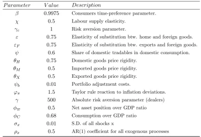
Instead of calibrating the parameters to a particular economy, we set the parameters to values that are standard in the new open economy literature, as shown in Table 1.1. The discount factor β is fixed at 0.9975, which implies a real interest rate of 1% in the steady state. The labour supply elasticity is set at 0.5 implying a relatively inelastic labour supply, though within the values found in empirical studies.24 The parameter

γ governing households’ risk aversion is fixed at 1, which is the one corresponding to logarithmic utility. The value for the elasticity of substitution between home and foreign goods is a controversial parameter. We follow previous studies in the DSGE literature, which consider values between 0.75 and 1.5.25 The share of domestic tradable goods in the CPI is set to 0.6, implying a participation of imported final and intermediate goods of 0.4 in the domestic CPI, in line with other studies for small open economies.26 Regarding price stickiness, we set a higher value for domestic goods over imported and exported ones. For domestic goods, the assumed stickiness implies that firms keep their

23_{A complete set of the log-linearised equations of the model can be found in Appendix 1.B.} 24

See Chetty et al. (2011).

25_{See Rabanal and Tuesta (2006). Other authors in the trade literature find values for this elasticity}

around 5, see Lai and Trefler (2002).

(34)

[image:34.595.121.521.126.399.2]

prices fixed for 4 quarters on average.

Table 1.1: Baseline Calibration

P arameter V alue Description

β 0.9975 Consumers time-preference parameter.

χ 0.5 Labour supply elasticity.

γc 1 Risk aversion parameter.

ε 0.75 Elasticity of substitution btw. home and foreign goods.

εF 0.75 Elasticity of substitution btw. exports and foreign goods.

ψ 0.6 Share of domestic tradables in domestic consumption.

θH 0.75 Domestic goods price rigidity.

θM 0.5 Imported goods price rigidity.

θX 0.5 Exported goods price rigidity.

ψb 0.01 Portfolio adjustment costs.

ϕπ 1.5 Taylor rule reaction to inflation deviations.

γ 500 Absolute risk aversion parameter (dealers)

φ$ 0.5 Net asset position over GDP ratio

φC 0.68 Consumption over GDP ratio

σx 0.01 S.D. of all shocks x

ρx 0.5 AR(1) coefficient for all exogenous processes

The parameter for portfolio adjustment costs is set a 0.01 to ensure that the cost of adjusting the size of the portfolio is small in the baseline calibration. For the central bank reaction function, we fixed a baseline reaction to inflation deviations of 1.5, which means that the central bank reacts more than one for one to inflation expectations, affecting the real interest rate. The coefficient of absolute risk aversion for dealers was set to 500 as in Bacchetta and Wincoop (2006).27 _{Finally, The standard deviation of}

all exogenous processes was set to 0.01 and the autocorrelation coefficient to 0.5. In the benchmark case, we calibrate the FX intervention reaction to exchange rate changes and real exchange rate misalignments to 0.5 for the ∆s rule and 0.3 for theRER rule, and analyse how results change with those parameters.

27

Notice that this parameter must be corrected by the steady state consumption level to make it comparable with the CRRA case. Additionally, only the product ofγ and the equilibrium value of the exchange rate volatility (of order 10−3)matterf orthemodeldynamics.

(35)

1.3.2 Model dynamics

In this section we present our results. We first discuss briefly the existence of equi-librium.28 Once we confirm the existence of an equilibrium, we study the effectiveness of different FX intervention strategies in reducing the macroeconomic volatility. We do this by contrasting the relative volatility of a sample of variables in the absence and under the presence of intervention. Next, we explore the reaction of the economy to external shocks under different intervention strategies through the calculation of impulse-response functions. We close this section studying how FX intervention affects the relative impor-tance of shocks to fundamentalsvis-`a-vis liquidity based trading. We present robustness exercises to the parameters defining the pass-through of exchange rates to prices (ε, εF)

and domestic price rigidity (θH in Section 1.4).

Rational expectations (RE) equilibria

As shown in Section 1.2, the risk premium-adjusted uncovered interest parity con-dition (equation 1.3) depends, among other things, on the concon-ditional variance of the change in the exchange rate. This, is an endogenous outcome of the RE equilibrium of the model. Solving for the RE equilibria entails solving for a fixed point problem in the conditional variance of the change in the exchange rate. In Figure 1-2, we plot the map-pings of the conjectured and the implied conditional variance of the depreciation rate for different parameterisations of the FX intervention reaction function. Intersections with the 45-degree straight line correspond to fixed points for the conditional variance of the depreciation rate.

As shown in the left-hand panels, there are two RE equilibria in the case of no FX intervention, corresponding to a low-variance stable equilibrium and a high-variance unstable equilibrium.29 This type of multiple equilibria is similar to the one found by Bacchetta and Wincoop (2006) in a model without FX intervention. However, as shown in the centre and right-hand panels, FX intervention helps to rule out the second unstable equilibrium. Under both rules of FX intervention there is only a unique and

28_{As in Vitale (2011), when solving for the equilibrium variance of the exchange rate, we are unable}

to rely on a theorem of existence, nor exclude the presence of multiple equilibria.

29_{A slope lower (higher) than one of the mapping of the conjectured and the implied conditional}

(36)

stable equilibrium. Also, the intensity of FX intervention reduces the RE equilibrium variance of the exchange rate change.30

The RE equilibrium variance of the exchange rate change also affects the direct impact of FX intervention and capital flows on the exchange rate, as shown in equation (1.3). Therefore, a more intensive FX intervention strategy also reduces its effectiveness as the reduction in variance dampens the impact of interventions on the exchange rate.

Transmission of external shocks

In Table 2 we present unconditional relative variances of some main macroeconomic variables assuming only one source of volatility at the time for different FX intervention regimes.31 For comparison, relative variances are normalised with respect to the no intervention case.

As shown, not surprisingly, FX intervention reduces the volatility of the change of the exchange rate in all cases. However, this exercise highlights some trade-offs in the use of FX intervention. In particular, the effects of FX intervention on the volatility of other macroeconomic variables will depend on the source of the shock. FX intervention helps to isolate domestic macroeconomic variables from financial external shocks, but amplifies fluctuations in some domestic variables from nominal and real external shocks.

For instance, the volatility of consumption, exports, output and inflation generated by foreign interest rate and capital flow shocks is reduced under both types of FX inter-vention regimes. However, the use of FX interinter-ventions to smooth the nominal exchange rate amplifies the volatility of inflation and output generated by foreign inflation shocks. Similarly, the use of a real exchange rate misalignment rule increases the volatility of con-sumption, exports, output and inflation generated by foreign output shocks. In this case, FX intervention prevents the adjustment of the real exchange rate as a macroeconomic stabiliser.

30_{This is a novel result, in stark contrast with the findings of Vitale (2011). We consider the author’s}

setup different to ours as in his model, central bank FX interventions are always informative and can potentially increase information dispersion across agents.

31

Exercises are simulated using the conditional variance of the depreciation rate in equilibrium in equation 1.3.

(37)

Figure 1-2: Existence of equilibria u nder FX in terv en tion rules (a) ∆ s rule ( ϕ∆ s = 0) 0 1 2 3 4 5 6 7 8 x 10 −3 0 1 2 3 4 5 6 7 8 x 10 −3

Conjectured Variance of Ex. Rate Depreciation

Implied Variance of Ex. Rate Depreciation

(b) ∆ s rule ( ϕ∆ s = 0 . 25) 0 1 2 3 4 5 6 7 8 x 10 −3 0 1 2 3 4 5 6 7 8 x 10 −3

(c) ∆ s rule ( ϕ∆ s = 0 . 50) 0 1 2 3 4 5 6 7 8 x 10 −3 0 1 2 3 4 5 6 7 8 x 10 −3

(d) R E R rule ( ϕr er = 0) 0 1 2 3 4 5 6 7 8 x 10 −3 0 1 2 3 4 5 6 7 8 x 10 −3

(e) R E R rule ( ϕr er = 0 . 25) 0 1 2 3 4 5 6 7 8 x 10 −3 0 1 2 3 4 5 6 7 8 x 10 −3

(f ) R E R rule ( ϕr er = 0 . 50) 0 1 2 3 4 5 6 7 8 x 10 −3 0 1 2 3 4 5 6 7 8 x 10 −3

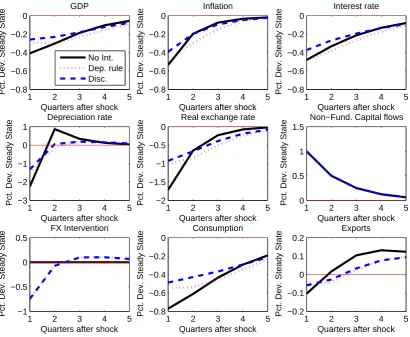
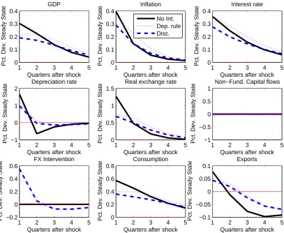
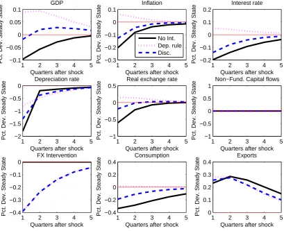
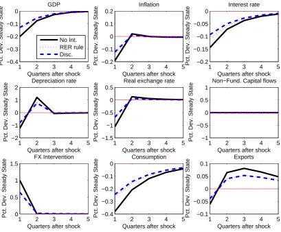
[image:37.595.123.527.76.754.2]

(38)

(39)

In Figures 1-3, 1-4 and 1-5 we compare the dynamic effects of external shocks under discretion, the ∆strule and the case with no intervention.32 Overall, the effectiveness of

intervention rules is confirmed. In other words, given that it is known the central bank will enter the FX market to prevent large fluctuations in the exchange rate, the amount of intervention necessary to reduce fluctuations is smaller. This means that the FX sales and purchases by the central bank necessary to stabilise the exchange rate will be much higher under discretion because it does not influence expectations as in the case of an intervention rule.

(40)

[image:40.595.119.530.98.435.2]

Figure 1-3: Reaction to a 1% portfolio shock - ∆st rule.

1 2 3 4 5

−0.8 −0.6 −0.4 −0.2 0 GDP

Quarters after shock

Pct. Dev. Steady State

No Int. Dep. rule Disc.

1 2 3 4 5

−0.8 −0.6 −0.4 −0.2 0 Inflation

1 2 3 4 5

−0.8 −0.6 −0.4 −0.2 0 Interest rate

1 2 3 4 5

−3 −2 −1 0 1 Depreciation rate

1 2 3 4 5

−2 −1.5 −1 −0.5 0

Real exchange rate

1 2 3 4 5

0 0.5 1 1.5

Non−Fund. Capital flows

1 2 3 4 5

−1 −0.5 0 0.5

FX Intervention

1 2 3 4 5

−0.8 −0.6 −0.4 −0.2 0 Consumption

1 2 3 4 5

−0.2 −0.1 0 0.1 0.2 Exports

Note: Intervention under discretion normalised to the implied intervention path under rules.

Contribution of shocks and FX intervention

Up to now we have shown the effectiveness of FX interventions by the central bank as a mechanism to cope with the effects of external shocks. To show this we have kept the variance of the exchange rate constant across regimes, as a way to make results comparable. However, as shown by Figure 1-2, intervention rules reduce the equilibrium value of the exchange rate volatility. This is key to understanding an additional effect of interventions. The impact of portfolio shocks on the exchange rate value is a function of the risk dealers bear for holding more foreign currency in their portfolio. Hence, a lower volatility will reduce the risk and consequently the premia they charge for these holdings. This makes interventions less effective when dealing with most external shocks, as shown by Table 1.2, while improving the resilience of the economy to portfolio or non-fundamental capital flow shocks. Specifically, when we assume the only shocks in the

(41)

[image:41.595.121.529.98.432.2]

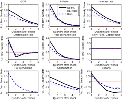
Figure 1-4: Reaction to a 1% foreign interest rate shock - ∆st rule.

1 2 3 4 5

0 0.1 0.2 0.3 0.4 GDP

1 2 3 4 5

0 0.1 0.2 0.3 0.4 Inflation

1 2 3 4 5

0 0.1 0.2 0.3 0.4 Interest rate

1 2 3 4 5

−1 0 1 2

Depreciation rate

1 2 3 4 5

0 0.5 1 1.5

Real exchange rate

1 2 3 4 5

−1 −0.5 0 0.5 1

1 2 3 4 5

−0.2 0 0.2 0.4 0.6 FX Intervention

1 2 3 4 5

0 0.2 0.4 0.6 0.8 Consumption

1 2 3 4 5

−0.1 −0.05 0 0.05 0.1 Exports

economy are given by the portfolio capital flows shocks, the volatility of the real exchange rate and the change of the exchange rate fall up to 85 and 87 percent respectively, in comparison to the no intervention case. This implies that through FX interventions, it is possible to reduce significantly the response of the exchange rate to portfolio shocks.33

Thus, our simulations show that intervention rules that reduce the volatility of the exchange rate affect as well the relative importance that shocks have in explaining this variance. In Figure 1-6 we show the variance decomposition of the exchange rate variation under different shocks. Our result is robust to the intensity of intervention, when the central bank intervenes in the FX market through rules, capital flows shocks explain a smaller fraction of the fluctuations of the change of the exchange rate, while the effect of others, such as foreign interest rate shocks, become relatively more important.

33

(42)

[image:42.595.120.530.252.585.2]

Figure 1-5: Reaction to a 1% foreign inflation rate shock - ∆strule.

1 2 3 4 5

−0.1 −0.05 0 0.05 0.1

GDP

1 2 3 4 5

−0.3 −0.2 −0.1 0 0.1

Inflation

1 2 3 4 5

−0.2 −0.1 0 0.1 0.2

Interest rate

1 2 3 4 5

−2 −1.5 −1 −0.5 0

Depreciation rate

1 2 3 4 5

−1 −0.5 0 0.5

Real exchange rate

1 2 3 4 5

−1 −0.5 0 0.5 1

1 2 3 4 5

−0.4 −0.3 −0.2 −0.1 0

FX Intervention

1 2 3 4 5

−0.4 −0.2 0 0.2 0.4

Consumption

1 2 3 4 5

0 0.1 0.2 0.3 0.4

Exports

(43)

Figure 1-6: V ariance decomp osition of the exc hange rate changes (∆ st ) (a) ∆ s rule 0 0.1 0.2 0.3 0.4 0.5 0 10 20 30 40 50 60 70 80 90 100

Intensity of intervention (change of ex. rate rule)

Variance decomposition (%)

Capital flows shock (contemp.) Foreign interest rate shock (contemp.) Other shocks and lags

(b) R E R rule 0 0.05 0.10 0.15 0.20 0.25 0 10 20 30 40 50 60 70 80 90 100

Intensity of intervention (real ex. rate rule)

Variance decomposition (%)

(44)

1.4

Robustness

We perform robustness exercises to several parameters related to the transmission mechanism of FX interventions into prices. Results are presented in Appendix 1.A. Results are robust to the assumed degree of elasticity between home and foreign goods (ε), as Tables 1.3 and 1.4 show. Tables 1.5 and 1.6 show results for changes in the elasticity of substitution between foreign and exports goods, (εF). This parameter has

strong effects on the capacity of the central bank to reduce the relative volatility of consumption and production in the face of financial shocks. This result is not surprising since a lower elasticity of substitution means that shocks to the exchange rate will have a smaller impact on the quantities exported, but a higher impact on the country’s income. As we observe, interventions are more effective reducing the volatility of consumption but less effective in the case of exports. The opposite occurs in the case of a high εF.

Tables 1.7 and 1.8 show results for the case of low and high domestic good price rigidity, respectively. We observe that price rigidity increases the effectiveness of FX intervention rules in isolating the economy from foreign interest rate shocks. Under low domestic good price rigidity, intervention rules imply a volatility of consumption between 43% and 96% of the no intervention benchmark. When price rigidity is high (θH = 0.95),

the relative volatility of consumption with intervention rules is between 12% and 64% of the no intervention benchmark. However, this result does not hold when the economy is hit by capital flows shocks. In this case, a central bank aiming to smooth the exchange rate can actually increase the volatility of variables such as consumption and production. The presence of high price stickiness, combined with a sluggish exchange rate - due to an active FX intervention policy - slows down corrections of the real exchange rate, increasing both consumption and GDP volatility.

1.5

Conclusions

In this chapter, we present a model to analyse the interaction between monetary policy and FX intervention by central banks, which also includes microstructure funda-mentals in the determination of the exchange rate. We introduce a portfolio decision of risk-averse dealers, which adds an endogenous risk premium to the traditional uncovered

(45)

interest rate condition. In this model, FX intervention affects the e