The London School of Economics and Political Science
Essays on Asset Pricing in Over-the-Counter Markets
Ji Shen
Declaration
I certify that the thesis I have presented for examination for the MPhil/PhD
degree of the London School of Economics and Political Science is solely my
own work other than where I have clearly indicated that it is the work of
others (in which case the extent of any work carried out jointly by me and any
other person is clearly identified in it).
The copyright of this thesis rests with the author. Quotation from it is
permitted, provided that full acknowledgement is made. This thesis may not
be reproduced without my prior written consent.
I warrant that this authorisation does not, to the best of my belief, infringe the
rights of any third party.
ABSTRACTS
The dissertation, which consists of three chapters, is devoted to exploring
theoretical asset pricing in over-the-counter markets.
In Chapter 1, I study an economy where investors can trade a long-lived asset in
both exchange and OTC market. Exchange means high immediacy and high cost
while OTC market corresponds to low immediacy and low cost. Investors with
urgent trading needs enter the exchange while investors with medium valuations
enter the OTC market. As search friction decreases, more investors enter the
OTC market, the bid-ask spread narrows and the trading volume in the OTC
market increases. This sheds some light on the historical pattern why most
trading in corporate and municipal bonds on the NYSE migrated to OTC markets
after WWII with the development of communication technology.
In Chapter 2 (co-authored with Hongjun Yan and Hin Wei), we analyse a search
model where an intermediary sector emerges endogenously and trades are
conducted through intermediation chains. We show that the chain length and the
price dispersion among inter-dealer trades are decreasing in search cost, search
speed and market size, but increasing in investors’ trading needs. Using data
from the U.S. corporate bond market, we find evidence broadly consistent with
these predictions. Moreover, as the search speed goes to infinity, our
search-market equilibrium does not always converge to the centralized-search-market
equilibrium. In particular, the trading volume explodes when the search cost
approaches zero.
In Chapter 3 (co-authored with Hongjun Yan), we analyse a search model where
two assets with different level of liquidity and safety are traded. We find that the
marginal investor’s preference for safety and liquidity is not enough to determine
the premium in equilibrium, but the whole distribution of investors’ valuations play
an important role. We specify the condition under which an increase in the supply
of the liquid asset may increase or decrease the liquidity premium. The paper
also endogenizes the investment in the search technology and conducts welfare
analysis. We find that investors may over- or underinvest in the search
Acknowledgements
CONTENTS
Chapter 1. Exchange or OTC Market: A Search-Based Model of Market
Fragmentation and Liquidity
1
Introduction ………..……….. 2
2
The Model ………...5
2.1 Value Functions ………..……….7
2.2 Demographic Analysis ……….… ……….9
2.3 Equilibrium ………..………….……… ……….11
2.4 Trading Volume ……… 17
2.5 Welfare Analysis ……… ………18
3
Discussions ……….……… ………20
4
Variation ……… ………..24
4.1 Investor’s Optimal Choice ………..………… ………25
4.2 Equilibrium ………..…….…… ……….27
5
Conclusion ………..……… ………31
6
Appendices ……… ………..34
Chapter 2. Financial Intermediation Chains in an OTC Market
1
Introduction ………..………….…… 82
2
Model ………..……….…… 88
2.1 Investors’ Choices ……….………..…….……… 89
2.2 Intermediation ………..……….…….. 91
2.3 Demographic Analysis ………..……….… 93
2.4 Equilibrium ………..………….… 94
3
Intermediation Chain and Price Dispersion ………..………..96
3.1 Search Cost
c
………..……….… 98
3.2 Search Speed
λ
……….……… 99
3.3 Market Size
X
……….……….. 99
3.4 Trading Need
κ
……… 100
3.5 Price Dispersion ……….. ……….100
3.6 Price Dispersion Ratio ……….… ……….…102
4
On Convergence ……….………..……….. 104
4.1 Centralized Market Benchmark ……….……… 104
4.2 The Limit Case of the Search Market ……….………105
4.3 Equilibrium without Intermediation ……….…....………108
4.4 Alternative Matching Functions ………..……….108
5
Empirical Analysis ……….………. 109
5.1 Hypotheses ……….…………..……….… 109
5.2 Data ……….………….………110
5.3 Analysis ……….………….……… …..112
6
Conclusion ……….………….……….114
7
Appendix ……….……….119
Chapter 3. A Search Model of the Aggregate Demand for Safe and Liquid
Assets
1
Introduction ………..……….…184
2
The Model ……… ……….…….189
2.1 Trading needs ……….………… 190
2.2 Demographics
……….………191
2.3 Value Functions ……….………193
2.4 Prices with Trading Frictions ……… 194
2.5 Equilibrium ………..………..… 195
2.6 The Liquidity Premium ……….…………..………….…198
2.7 Trading Needs and Asset Prices ……….………..…… 201
2.8
Welfare
……….…… 202
3
The Safety Premium ……….… 204
4
Conclusion ……….… ………..207
5
Appendix ……….… ……….…210
Exchange or OTC Market: A Search-Based Model of
Market Fragmentation and Liquidity
Abstract
1
Introduction
Nowadays, many commodities and assets can be traded simultaneously in both centralized ex-change and decentralized over-the-counter (OTC) markets. For example, Chinese enterprise bonds are traded in two partially-separated markets, the exchange and the interbank market (Wang et al, 2015). Multiple trading venues meet di¤erent levels of traders’needs: exchange usually means high immediacy and high cost while OTC market, however, corresponds to low immediacy and low cost. How do these two markets interact with each other? What factors determine liquidity, trading volume and bid-ask spread in each market and how? How can a decentralized solution be compared with the socially optimal solution? These are the basic questions we attempt to answer in this paper.
We study an economy where investors can trade a long-lived asset through two trading venues: exchange or OTC market. Transactions in the exchange can be executed instantly, but incur some explicit costs. Trading in the OTC market incurs time delay. Investors are heterogenous in their intrinsic valuations of the asset and each one’s valuation changes over time, which generates trading between people and across time. Investors are free to enter either market. In this sense, the two trading venues are linked together to some degree, so the pricing in one market a¤ects trading activity in the other.
The model in Section 2 extends the seminal work of Du¢ e, Garleanu and Pedersson (2005, 2007) by enriching investor heterogeneity and incorporating a centralized market, but an individ-ual investor’s valuation spans over interval 0; . For simplicity, we still assume that each investor can hold either one unit of the asset or no unit at all. Investors with desperate trading needs directly go to the exchange while those with intermediate trading needs enter the OTC market. More precisely, given that transaction cost in the exchange is not very big so that both markets are active in trading, there exist three cuto¤ points, 0, w and 1, with 0< 1 < w < 0 < .
Non-owners with high valuations (i.e., 2 0; ) choose to buy in the exchange, those with
(i.e., 2( w; 0)) choose to search in the OTC market. The optimal decision-making for
own-ers also follows a simple cuto¤ rule. Ownown-ers with low valuations (i.e., 2 [0; 1]) choose to
sell in the exchange, those with intermediate valuations choose to sell in the OTC market (i.e.,
2( 1; w)) and those with high valuations (i.e., 2 w; ) choose to hold onto the asset.
Investors’entry choices determine that the bid (or ask) price in the exchange should be charged more aggresively than their counterparts in the OTC.
To further determine the bid-ask spread, we analyze two extreme cases of market making in the exchange: competitive or monopolistic. The bid-ask spread in the exchange set by a monopolistic market maker becomes narrower if search friction in the OTC is alleviated, if investors’trading needs are stronger or if investors become less patient. Interestingly, we also …nd that how the asset supply a¤ects the bid-ask spread is somehow related to the shape of the underlying valuation distribution.
We specify the conditions under which both markets can coexist or all trading just occurs to only one market. Generally speaking, the relative e¢ ciency of the two markets (including trans-action costs and search friction) and investors heterogeneity mutually determine the boundary of market trading.
A quite robust observation from empirical studies is that the average trading volume in the OTC market is much bigger than that in the exchange. In Section 2.4, we compare trading volumes in two markets and …nd that an improvement of search technology in the OTC market attracts more investors to trade in the OTC. This may shed some light on the historical pattern that, with the development of communication technology, most trading in corporate and municipal bonds on the NYSE have migrated to OTC markets after World War II.
We perform welfare analysis in Section 2.5. A benevolent social planner aims to maximize the total welfare by controlling asset prices in both markets. We …nd that the social planner tends to set a low 0 and a high 1 relative to the decentralized solution under competitive or
the transaction cost. This means that the social optimum can not be automatically achieved by a competitive equilibrium where market makers in the exchange receive no subsidy from outside.
Though the main model provides several useful intuitions and important implications, its tractability relies heavily on the strong assumptions of asset indivisibility and restrictions on investors’holding position. Will the main results di¤er a lot if we deviate from these two assump-tions? In Section 4, we work on a variation where the asset is perfectly divisible and investors are allowed to trade any quantity. The new model is more complicated than the old one and there could exist multiple equilibria. In a special case when the investor’s instantaneous utility takes a quadratic form, we …nd that the bid-ask spread in the exchange takes almost exactly the same expression as before.
This paper is related to the recently burgeoning literature that uses random search model to analyze OTC markets. The strand of this literature is based on the framework developed in Du¢ e, Garleanu and Pederson (2005). Their model has been generalized by a number of papers (Weill (2007), Vayanos and Wang (2007), Vayanos and Weill (2008), etc). The closest to the current paper is Miao (2006), who also analyzed a model where decentralized and centralized trading are both available. The current paper is di¤erent from his work in a number of important ways. Most importantly, in contrast to Miao’s paper, this work analyzes an environment where a long-lived asset are traded repeatedly in the market, so buyers and sellers are endogenously determined rather than exogenously …xed. However, in Miao’s model, when trade occurs to a pair of seller and buyer, they both leave the market forever. The paper also draws di¤erent welfare implications from Miao’s. Miao showed that monopolistic market-making may achieve a higher level of social welfare than the case of competitive market-making, which can never be the case in the current framework. A recent work by Zhong (2015) also analyzes the interaction between centralized and OTC market, but his work focuses on how the introduction of centralized trading reduces opacity in the OTC market, which is not the focus of this paper.
restrictions on portfolio holdings are relaxed.
2
The Model
Time is continuous and continues forever. The economy consists of three types of in…nitely lived agents, called investors, dealers in the OTC market and market makers in the exchange. All agents are risk neutral and discount future cash ‡ow at a constant rater >0. There are an asset available for trading and a numeraire good for consumption in the economy.
The asset is long-lived and indivisible. Each unit of the asset pays one unit of perishable consumption good continuously to its holder. Each investor can hold either zero or one unit of the asset and no short-selling is allowed. An investor who owns a unit of the asset is called an owner while one with no asset in hand is called a non-owner.
Each investor, whether he is an owner or a non-owner, has an intrinsic valuation for the asset, denoted by 2 ; . An owner derives an instantaneous utility 1 + from the asset if his current intrinsic valuation is . A non-owner, however, gets zero consumption good, no matter what his valuation is.
position in the asset, so all units are held by investor at any point of time.
OTC market. Dealers have direct access to a competitive interdealer market continuously. It takes time for investors to contact dealers. Each investor meets a dealer randomly at a Poisson arrival rate >0, i.e., the average time that an investor has to wait until his desired transaction is executed is 1= . Once a dealer meets a buyer (or seller), they exchange one unit of the asset at bid price PA (or ask price PB). The bid-ask spread, PA PB, is used to cover the cost of
intermediating each unit of the asset incurred by the dealer. Denote such cost by . Free entry implies
PA PB= : (1)
Both of the bid and ask prices are determined in the interdealer market. Here, parameter measures the illiquidity of the OTC market from investors’viewpoint. A large translates to a short delay time and thus corresponds to a liquid market. When goes to in…nity, investors can adjust their asset positions instantaneously. 1
Our formulation for search friction in the OTC market can also be understood as prearranged trades, which are often seen in the municipal bond market. An investor calls a dealer to show his trading interest. The dealer then searches for a counterparty. Once the dealer has found a trading partner, he transfers the bond from the seller to the buyer. Hence, the dealer’s role in a pre-arranged trade is simply to provide intermediation service. 2 In this interpretation, the parameter measures how quickly a dealer position a trading partner for his client.
Throughout, we will stick to the …rst interpretation, but it is direct to rephrase our results in the second interpretation.
Exchange Market. At any time, each investor can buy the asset at ask price A and sell the asset at bid priceB immediately. Both of the bid and ask prices are observed publicly by all market participants, including all investors and dealers in the OTC market. A transaction incurs 1Here we take as exogenously given. In Section 4, we will discuss how to determine this parameter endogenously. 2
a …xed cost c.
For time being, we assume that there is active trading in both markets. We will later show the condition under which this is the case or one of the two markets shut down due to no trading otherwise.
An investor is free to enter either of the two trading venues at any moment and there is no cost for him to switch one from the other. Even if an investor in the OTC market gets a chance to contact a dealer, he can still choose to trade in the exchange. Hence, the following condition should hold in equilibrium to guarantee active trading in both markets:
A > PA> PB > B: (2)
Otherwise, if the prices in the OTC market are not particularly favorable, all investors would rather trade in the exchange.
2.1 Value Functions
The state of an individual investor is characterized by the pair( ; ), where 2 f0;1gis his asset position and his intrinsic valuation. Let V( ; ) be the expected payo¤ of such an investor.
A non-owner faces two choices: 1) do nothing, 2) search to buy the asset in the OTC, 3) buy a unit of asset in the exchange at price A. He decides to choose the one that delivers him the highest level of the expected payo¤, i.e.,
V (0; ) = maxnVn( ); VbOTC( ); V
exchange
b ( )
o
; (3)
where Vn( ), VbOTC( ) and Vbexchange( ) represent the non-owner’s expected payo¤s if he
are determined by the following equations
Vn( ) =
+rE V 0;
0 ; (4)
VbOTC( ) = [V (1; ) PA] + E[V (0;
0)]
+ +r ; (5)
Vbexchange( ) = V (1; ) A; (6)
where the expectations on the …rst two lines are taken on 0, which is a random variable with cdf F( ). The …rst line says that a non-owner who chooses not to search stays inactively until he receives a shock in his valuation which may call upon him to buy the asset. It is direct to see that
Vn( ) is constant for all , so we denote it by Vn. The second line shows that a buyer in the
OTC keeps searching until he meets a dealer and purchase one unit at price PA, which happens
at rate , or there is a change in his valuation and he needs to make a decision based on his new valuation. The third line illustrates that a buyer in the exchange becomes an owner immediately after he pays A.
An owner has three choices: 1) hold onto his asset, 2) search to sell the asset or 3) sell the asset in the exchange immediately, so the expected payo¤ of an owner should be given by
V(1; ) = max
n
Vh( ); VsOTC( ); Vsexchange( )
o
; (7)
whereVh( )represents the expected payo¤ of an inactive holder andVsOTC( )andV
exchange
s ( )
are the non-owner’s expected payo¤s if he searches to sell the asset in the OTC or sells the asset in the exchange at present and follows his optimal strategy in his whole life, respectively. These three value functions are given by
Vh( ) =
1 + + E[V (1; 0)]
+r ; (8)
VsOTC( ) = 1 + + [V (0; ) +PB] + E[V (1;
0)]
+ +r ; (9)
Vsexchange( ) = V(0; ) +B; (10)
where the expectations on the …rst two lines are taken on 0, which is a random variable with cdf
We will later verify that in equilibrium a non-owner follows the following optimal decision
rule: 8
< :
do nothing if 2[ ; )
search to buy the asset in the OTC if [ ; 0]
buy the asset in the exchange if 2 0;
; (11)
where and 0 are two cuto¤ points to be determined in equilibrium. A non-owner is indi¤erent
between doing nothing and searching in the OTC if his valuation is and is indi¤erent between trading in the OTC and the exchange market if his valuation is 0:
Vn( ) = VbOTC( );
VbOTC( 0) = Vbexchange( 0):
There exist another two cuto¤ points and 1 with 1 < such that an owner’s
optimal choice is given by 8 < :
sell the asset in the exchange if 2[ ; 1)
search to sell the asset in the OTC if [ 1; ]
hold onto the asset if 2 ;
; (12)
where 1 and satisfy
Vsexchange( 1) = VsOTC( 1);
VsOTC( ) = Vh( ):
That is, the marginal owner with valuation 1 is indi¤erent between selling in the exchange and
the OTC market while the marginal owner with valuation is indi¤erent between searching to sell in the OTC and holding onto his asset.
We now brie‡y argue . Suppose not, i.e., < and consider the behavior of a buyer with valuation in the interval ( ; ). As a non-owner, he searches to buy the asset in the OTC according to decision rule (11). Once he buys the asset after paying PA, he would
turn to sell the asset still in the OTC, according to decision rule (12), at a somewhat low price
PB. Such an investor actually acts as a speculator, but his strategy is to "buy high and sell
All in all, the four cuto¤ points should be ordered as
1 < < 0:
2.2 Demographic Analysis
We use o( ) and n( ) to denote the density function of owners and non-owners at re-spectively, i.e., the population size of the owners (or non-owners) with valuations in the region
( ; +d ) is o( )d (or n( )d ). The following accounting identities must hold for any time:
o( ) + n( ) = f( ); (13)
Z
o( )d = s: (14)
Equation (13) means that the cross-sectional distribution of investors’ type is equal to f( ). Equation (14) requires that the total measure of owners must equal to the total supply of the asset in the economy (s) because both of the exchange and the OTC market take zero asset position. This implies
Z
n( )d = 1 s:
Since trading in the exchange results in no delay, decision rules(11) and(12)then imply that
o( ) = 0 for 2[ ; 1);
n( ) = 0 for 2 0; :
It follows immediately from (13) that
n( ) = f( ) for 2[ ; 1);
o( ) = f( ) for 2 0; :
We next determine o( )and n( )for 2[ 1; ]. For this, we consider the ‡ows in and
period dt. According to(12), these sellers search in the OTC. The in‡ow is dt sf( ), coming from those sellers who receive preference shocks and whose new valuations happen to fall in this interval. The out‡ow consists of those sellers who meet dealers and trade ( dt o( )), and of those sellers who receive preference shocks ( dt o( )). The ‡ow-balance equation is thus given by
sf( ) = o( ) + o( ) for 2[ 1; ]:
Using the similar logic, we can …gure out o( ) and n( ) for 2( ; ) and [ ; 0].
For the sake of saving space, we relegate all the details to the appendix.
Since the dealer sector, as a whole, holds no inventory, it follows that the mass of buyers should equal that of sellers, namely,
s = b; (15)
where the masses of buyers and sellers are given by, respectively,
b =
Z o
n( )d ; (16)
s =
Z
1
o( )d : (17)
The market makers in the exchange hold no position either. According to seller’s decision rule (12), the total number of units sold from low-valuation investors to the exchange per unit time amounts to sF( 1). According to buyer’s decision rule (11), the total number of units
demanded by high-valuation investors per unit time is given by (1 s) [1 F( 0)]. In the
exchange, the demand equals the supply at any time, so
sF( 1) = (1 s) [1 F( 0)] (18)
2.3 Equilibrium
De…nition 1 GivenAandB, the steady-state (partial) equilibrium consists of bid and ask prices in the OTC PA andPB, cuto¤ points 1; ; and 0 with 1 < < 0 , the distributions of owners and non-owners ( o( ); n( )), such that
the implied choices (11) and (12) are optimal for all investors,
the implied sizes of each group of investors remain constants over time and satisfy the corresponding ‡ow-balance equations,
dealers are free to enter the OTC market, i.e., (1) holds,
the market-clearing conditions in the OTC and exchange market, (15) and (18), hold.
Our analysis will be focused mainly on the case of = 0, with the only exception in Section 4 where we analyze the impact of dealer’s transaction cost on asset prices. When = 0, the wedge between the bid and ask prices in the OTC market vanishes, so PA = PB, which we denote by
P. We show in the appendix that this leads to = . In what follows, when we mention "bid-ask spread", it always refers to the one in the exchange as there is no such thing in the OTC market.
The following proposition characterizes a steady state equilibrium.
Proposition 1 (Partial equilibrium with = 0) If c A B < + +r, the steady-state partial equilibrium given A and B is the following. The cuto¤ points are given by
= = w; (19)
and 0 and 1 are uniquely determined by the following equations
A B = 0 1
+ +r; (20)
(1 s)F( 0) +sF( 1) = 1 s: (21)
The asset price charged by the dealers in the OTC market, P, is given by
P = 1 + w
r r
R w
1 F( )d
+ +r + r
R 0
w[1 F( )]d
Investors’ distributions are given by
n( ) =
8 > > > < > > > :
f( ) for 2[ ; 1) (1 s)+
+ f( ) for 2[ 1; w) (1 s)
+ f( ) for 2[ w; 0]
0 for 2 0;
; (23)
and
o( ) =
8 > > > < > > > :
0 for 2[ ; 1)
sf( )
+ for 2[ 1; w)
s+
+ f( ) for 2[ w; 0]
f( ) for 2 0;
: (24)
Equation(20)shows that the distance between 0 and 1 is positively related to the bid-ask
spread and negatively related to investor’s e¤ective discount rate. Recall that in equilibrium only those buyers with valuation above 0 and sellers with valuation below 1 choose to trade in the
exchange, so the distance between these two cuto¤ points gives the range of investors who are active in the OTC market and therefore re‡ects the bid-ask spread in the exchange. Equation
(21) just highlights that no asset is held in the hand of market makers, a copy of constraint(18).
The asset price in the OTC market in(15)consists of three components. The …rst part, 1+ w
r ,
is exactly the asset price in the frictionless benchmark. It re‡ects the present value of the cash ‡ow for the marginal investor with valuation w. The second term captures the buying pressure
on the price. Recall that sellers in the OTC, with valuations ranging from 1 to w, would like
to sell at a low price if they have to wait for a long time. The third term corresponds to the selling pressure, imposed by buyers in the OTC, whose valuations range from w to 0.
In the literature, trading volume is an important measure of liquidity. The total units of the asset being traded in the exchange is given by
TVexchange = sF ( 1); (25)
and the total units of the asset being traded in the OTC market is given by
TVOTC = b =
s
+ [1 s F( 1)]: (26)
We will compare them in Section 2.4. For any …nite , the total trading, which is the sum of
benchmark. 3
In general, there are three types of equilibria. If < 1 < w < 0 < , the two markets
coexist. If 1 = and 0 = , there is no active trading in the exchange and only the OTC
market survives. If 1 = 0 = w, the OTC market is quiet and only the exchange market
survives. We will later show that the last situation could never be the case in equilibrium unless
= 0. 4
In order to determine the equilibrium, we need to specify how the bid and ask prices in the exchange are set up. For this, we consider two cases of market structure in the exchange. In the …rst case, free entry induces perfect competition among market makers. The second case is monopolistic market making.
Competitive Market Making. Fierce competition among market makers in the exchange should drive the average pro…t down to zero, so the bid-ask spread can only cover the cost of making market for each share, i.e., A B =c.
We …rst have the following result.
Proposition 2 Consider the search equilibrium with competitive market makers in the exchange. If ( + +r)c < , trading occurs to both the exchange and the OTC market.
This proposition establishes that if either the cost of market making or the e¤ective discount rate is high enough, all investors prefer to trade in the OTC market and there is no active trading in the exchange.
3
This can be easily seen from
TVe x ch a n g e+TVO T C =
+ sF( 1) + + s(1 s)
<
+ s(1 s) + + s(1 s)
= s(1 s) =TVW a lra s ia n;
where we use 1< w in the second step.
4
To show an example, we assume F( ) is a uniform distribution on 0; . In this case, the Walrasian cuto¤ point is given by w= (1 s) . The two cuto¤ points, denoted by c0 and c1
speci…cally, are given by
c
0 = min (1 s) +sc( + +r); ;
c
1 = max (1 s) (1 s)c( + +r);0 :
The asset price in the OTC market, denoted by PCM speci…cally, is given by
PCM =
8 < :
1+(1 s)
r +
c
r (2s 1) 1
( + +r)c
2 , if ( + +r)c < 1+(1 s)
r + r
(s 12)
+ +r, if ( + +r)c
: (27)
(27) illustrates that PCM consists of three components. The …rst term in PCM is actually
Pw, the Walrasian price of the asset in the frictionless benchmark. It is obvious to see that
whether PCM is above or below its Walrasian counterpart depends solely on the asset supply. If
s > 12, there are more owners than non-owners in the economy and the buying pressure dominates which pushes PCM up to overtake Pw. If s < 12, there are more non-owners than owners in the
economy and thus the selling pressure dominates, which results inPCM < Pw. In both cases, an
improvement in the search technology (which corresponds to a higher level of ) enables PCM to approach Pw. Whens= 12, the two pressures are in balance.
Monopolistic Market Making. A monopolistic market maker sets upAandBto maximize his expected pro…t. In the steady-state equilibrium, the pro…t per unit time is given by
(A B c)TVexchange= s 0 1
+ +r c
1
;
subject to the constraint that the market maker holds zero inventory in his hand, i.e.,
(1 s) 0 +s 1 = 1 s:
Proposition 3 The search equilibrium with a monopolistic market maker is characterized as follows. If ( + +r)c < , trading occurs to both the exchange and the OTC market. If
denoted by m0 and m1 speci…cally, are given by m
0 = min
n
1 s
2 +
s
2( + +r)c;
o
;
m
1 = max
(1 s)
2
1 s
2 ( + +r)c;0 :
The asset price in the OTC market, denoted by PM M speci…cally, is given by
PM M =
8 < :
1+(1 s)
r + r c+ + +r s
1 2
3 4
( + +r)c
4 , if ( + +r)c
1+(1 s)
r + r
(s 12)
+ +r, if ( + +r)c >
:
If ( + +r)c < , the bid-ask spread in the exchange is given by
A B =
2 ( + +r) +
c
2: (28)
The bid-ask spread increases inc and and decreases in the e¤ective discount rate. First, a unit increase in transaction costctranslates into a partial increase in the bid-ask spread. Note that increasing the bid-ask spread also discourages some investors from trading in the exchange and results in a decreased demand for the monopolistic market maker. Second, if investors are more dispersed in their valuations, then a wider bid-ask spread is charged. Third, a higher discount rate also leads to fewer investors to trade in the exchange, so the market maker has to narrow the bid-ask spread to maintain his business.
We will see in Section 5 that all the above results of comparative statics still hold in the case when asset is divisible and investors are allowed to hold and trade any amount. Interestingly, the bid-ask spread (for each share) in the new equilibrium takes exactly the same expression as here if investor’s instantaneous utility is quadratic.
Note that the asset supply (denoted by s) does not play an explicit role in (28), though it does a¤ect m0 and m1 . The absence of s in determining the optimal bid-ask spread is due to the speci…cation of F( ). The following two numerical examples indicate that the shape of the underlying preference distribution is an important factor to determine the supply e¤ect on the bid-ask spread.
Example 2. IfF( ) = 2 on [0;1], the bid-ask spread increases in s.
2.4 Trading Volume
According to an empricial research on the Chinese bond markets (Wanget al, 2015), trading takes place more frequently in the exchange but the average transaction size there is much smaller than that in the OTC market. The average trading volume in the OTC market is over thirty times more than that in the exchange. In the current model, the transaction size for each trade is restricted to be one, so the number of trades equal the total trading volume then. We check whether this simple model captures this important pattern.
The following table summarizes how the cuto¤ points and trading volume in each market respond to the change in some underlying parameters under competitive market making.
Table: Comparative Statics Results
0 1 TVexchange TVOTC
" " # # "
c" " # # " r" " # # "
" " # ? "
The …rst two lines are easy to understand. When the exchange becomes relatively more costly, which is captured by an increase in orc, more investors are willing to trade in the OTC market. When investors are more impatient, which translates to a highr, holding an asset is less valuable. This makes the delay cost in the OTC market less intolerable, so more investors are attracted to the OTC market, as we see on the third line. The e¤ect of on the cuto¤ points is clear. The higher is, more frequenly an investor’s type changes. This has two e¤ects. On the one hand, it shortens the holding period of an asset for an owner and thus makes waiting in the OTC market less costly. This surely widens the distance between 0 and 1 and increases TVOTC, but does not lead to a lower TVexchange because a higher also implies that more investors want to trade during each instant.
Proposition 4 Suppose F( ) = for 2 0; and ( + +r)c < . There exist positive valuesr0; c0and 0 such thatTVOTC >TVexchange ifr > r0, orc > c0 or > 0 under competitive market making. Similar results obtain under monopolistic market making.
Note that we haven’t mentioned the role of as it may increase the trading volumes in both markets.
2.5 Welfare Analysis
In this subsection we examine whether the bid-spread, determined in Subsection 2.3, is socially optimal.
The social welfare in the search equilibrium is de…ned as the sum of all investors’ expected payo¤s and total pro…ts for market makers:
Wd=
Z
[V (0; ) n( ) +V (1; ) o( )]d +1
r(A B c)TVexchange: (29)
Since the type distribution for investors in a steady-state equilibrium does not change over time, we can also consider the realized surplus per period, which is the sum of the total consumption goods received by all owners net of total transaction costs in the exchange, i.e.,
Ws=
Z
(1 + ) o( )d c TVexchange: (30)
Here, the subscriptdin(29)stands for "dynamic" and the subscriptsin(30) stands for "static".
It is easy to see that the social planner tends to allocate the desperate investors to the exchange and investors with medium trading motives to the OTC market, so the optimal allocation rule of investors should take a similar cuto¤ form as in (12) and (11). The following proposition summarizes the socially e¢ cient allocation.
Proposition 5 Maximizing the welfare criterion in (29) and (30) lead to the same solution of social optimum, which is characterized by the following. (I) There exist two cuto¤ points, denoted by f b0 and f b1 , such that (i) if( + )c < , f b1 is the unique solution to the following equation
(1 s)F f b1 + ( + )c +sF f b1 = 1 s,
and f b0 = f b1 + ( + )c, (ii) if ( + )c , s0 = and s1 = 0. (II) An owner’s
optimal choice is given by (12) and a non-owner’s optimal choice is given by (11), where we set
= = w and replace 0 by f b0 and 1 by f b1 therein. (III) If ( + )c , trading occurs to the OTC market but not the exchange. If ( + )c < , trading occurs to both the exchange and the OTC market and the bid-ask spread in the exchange is given by ( + )+ +cr.
Here, the superscriptfb stands for "…rst-best". The condition to have active trading in both markets in the social optimum isc < + . Recall that the corresponding condition in the decen-tralized solutions in Proposition 2 and Proposition 3 is c < + +r. Note that the value of f b0 and f b1 are independent ofr. This is obvious if we use the static welfare criterion because there is no r in(30), but not so obvious if we use the dynamic welfare criterion.
We …nd that the socially optimal bid-ask spread in the exchange is strictly below the required transaction cost. This means that the social optimum can not be sustained even by a competitive equilibrium unless the market makers in the exchange receive some subsidy from outside.
Proposition 6 If c < + +r, the cuto¤ points in all three equilibriums are ranked by m
0 > c0>
f b
0 >
f b
1 >
c
1 > m1 :
If + +r c < + , they are ranked by m
0 = c0 = >
f b
0 >
f b
If c + , then m
0 = c0 =
f b
0 = and c1 = m1 =
f b
1 = 0.
Note that a higher level of 1 and a lower level of 0 mean that investors with a larger
range of valuations are trading in the exchange. Given the transaction cost is not very large, the social planner’s main concern is focused on the delay cost paid by those investors waiting in the frictional OTC market. This proposition says that the search equilibrium under monopolistic market making keeps too many investors away from the exchange, so they have to wait in the OTC market and bear a large amount of delay cost. Such deadweight loss will be re‡ected in the aggregate welfare.
Finally, we are ready to compare the total welfare across di¤erent equilibriums. Denote for short the social welfare in the search equilibrium under competitive market-making and monop-olistic market-making by WCMd and WM Md , respectively. Denote the social welfare in the social optimum by WF Bd . The following result con…rms that neither the social welfare under monopo-listic market-making nor that under competitive market-making could achieve the social optimal level because they just allow too few investors to trade in the exchange.
Proposition 7 If c < + +r, then WF Bd >WCMd >WM Md . If + +r c < + , then WF Bd >
WCMd =WM Md . Ifc + , then W
F B
d =WM Md =WCMd .
3
Discussions
In this section, we discuss some further issues.
Endogenous Determination of Search Intensity . So far, we have taken as ex-ogenously given. It is easy to determine this parameter by assuming a matching function. Let d be the mass of dealers and still use b and s to denote the mass of buyers and sell-ers, respectively. The number of dealer-buyer pairs being matched per unit time is given by
M( b; d)= d = M( b= d;1) m( b= d), where m( ) is a strictly increasing function. Sim-ilarly, the number of dealer-seller pairs being matched per unit time is given by M( d; s). A seller meets a dealer at rateM( s; d)= d=m( s= d). Since the dealers do not hold inventory, we have s= b. Hence, is given by
=m( b= d): (31)
Here, b is also determined in the equilibrium endogenously. In the appendix, we show
b =
(1 s)
+ [F( 0) (1 s)]:
Note that a¤ects b in two opposite directions. On the one hand, an increase in means a high speed of matching and a shorter expected time delay, resulting in fewer searchers in the OTC market. This e¤ect is re‡ected by the in the denominator of the above expression. On the other hand, a reduction in the search friction attracts more investors to enter the OTC market. This e¤ect is captured by 0, which is expected to be increasing in . When F( ) is uniform, the …rst
e¤ect dominates and b is decreasing in under monopolistic or competitive market-making.
It follows that the RHS of (31) is decreasing in while the LHS of this equation is obviously increasing in . It is then easy to show that a unique exists.
Positive Cost of Market-Making in the OTC Market: > 0. We construct the equilibrium for a positive in Theorem 1 in Appendix I. Comparing with the special case of = 0
reported in Proposition 1, we highlight three di¤erences. First, unlike (19), there is now a wedge between and :
= ( +r) :
Second, the bid-ask spread in the exchange and the type range are now governed by
A B= 0 1+
+ +r ; (32)
which is a generalization of (20). Third, the bid-ask spread in the OTC market equals , i.e., (1).
If > 0> > > 1>0, both markets are active.
If > 0= = 1>0, trading only occurs to the exchange.
If = 0> > 1= 0, trading only occurs to the OTC market.
If = 0> and = 1 = 0, no trading occurs to either market.
The following proposition analyzes which market is active in trading under competitive market making.
Proposition 8 Consider the search equilibrium with competitive market makers in the exchange. If c +r, no trading occurs to either market. If < c < + ++ r, active trading occurs to both markets. If c + ++ r > , trading only occurs to the OTC market. If c= < +r, active trading only occurs to the exchange.
The following proposition reports the impacts of on the equilibrium.
Proposition 9 Consider the search equilibrium with competitive market makers in the exchange. (I) When c, 0 = 1 = w, i.e., there is no active trading in the OTC market. (II) When
< c, 0 and 1 are uniquely determined by (21) and (32). As increases, more investors choose to trade in the exchange, i.e., @ 0
@ <0< @ 1
@ , @ b
@ >0 and
@TVexchan ge
@ >0>
@TVO T C
@ .
The results in Proposition 8 and 9 hold for a general cumulative distribution F( ). Part (I) of Proposition 9 reveals that the OTC market is driven out of the economy if is large relative toc. In this case, intermediating transactions in the OTC market is too costly relative to market making in the exchange, so all trading activities migrate to the exchange.
Consequently, decreases TVOTC and increases TVexchange. An interesting observation is that increases the total trading volume. This means the increase in TVexchange is more than the decrease in TVOTC.
As for the equilibrium with a monopolistic market maker, we carry out the same analysis as in Proposition 3 and obtain the optimal bid-ask spread:
A B = +
2 ( + +r) +
c
2:
Several points are in order. First,A B is increasing in . This is because when is increased, the advantage of the exchange over the OTC market becomes larger and raising the bid-ask spread does not lose but win more business for the market maker. Second, all of the comparative statics results still hold and the intuitions are similar. Just like the case of = 0, the bid-ask spread is still positively related to ,c and negatively related to ,r and .
In addition, we can decompose the bid-ask spread in the exchange into three components:
A B = (A PA) + (PA PB)
| {z }
= according to(1)
+ (PB B);
where the term in the …rst (or last) bracket is the spread of ask (or bid, respectively) price between two markets and the term in the middle bracket is the bid-ask spread in the OTC market. 5 The increase of narrows (A PA) and (PB B).
The following proposition analyzes which market is active in trading under monopolistic mar-ket making.
Proposition 10 Consider the search equilibrium with a monopolistic market maker in the ex-change. Assume F( ) is uniform on 0; . Both markets are active if 1 + +r c < <
+( + +r)c
+2( +r) . Trading only occurs to the exchange if
+( + +r)c
+2( +r) < +r. Trading only occurs to the OTC market if <max
n
+( + +r)c
+2( +r) ; 1 +
+r c o.
5More precisely, both (A P
A) and(PB B) are positively related to and cand negatively related to the
4
Variation
In this section, we consider a model in which the asset is divisible and investors are allowed to hold and trade any amount of quantities, though short-selling is still not allowed. Basically, we extend the search model in Lagos and Rocheteau (2009) by adding a centralized exchange.
The instantaneous utility function of an investor is ui(q) +c, where q 0 represents the
investor’s asset holdings, c is the net consumption of the numeraire good and i2 f1;2g indexes his preference shock. Note that a non-negative q means short-selling is forbidden, but c can be positive or negative. To get closed-form solutions, we will mainly employ a quadratic utility function in this section:
ui(q) = iq
1 2q
2; (33)
where 2> 1>0. This speci…cation of utility is obviously strictly increasing and strictly concave
inq. A bigger i translates to a higher level a marginal utility. Each investor receives a preference
shock with Poisson arrival rate . Conditional on receiving such shock, the investor draws i with
probability i >0, where 1+ 2 = 1.
OTC market. Investors contact dealers randomly at arrival rate . Once a dealer and an investor meet each other, they negotiate over the terms of trade, which now consist of the quantity of assets that the investor aims to exchange and the intermediation fee that the dealer charges for his services. The two parties split total trade surplus via Nash bargaining, that is, the dealer gets fraction of the trade surplus and the investor gets the remaining fraction. We still use P
to represent the asset price for each unit in the OTC market, whose value should be determined in equilibrium.
Exchange. This is the same as before, i.e., investors can enter the exchange at any point of time and buy (or sell) any quantity of the asset at unit ask priceA (or unit bid priceB).
quantity of assets as the net holdings in their portfolios are non-negative. Second, investors and dealers in the OTC market bargain over the price and quantity at the same time. As long as dealers have a strictly positive bargaining power, i.e., 2 (0;1], they can earn some positive intermediation fees.
4.1 Investors’Optimal Choice
An investor with preference type i and asset holdingq is indexed by a pair (i; q)2 f1;2g R+,
which is called as his state in what follows. Let i(q) denote the value function of such an
investor, i.e., the maximum expected utility attained by an investor of type (i; q).
Suppose an investor in state (i; q) chooses to enter the OTC market and let Ui(q) be the
expected discounted utility for him. Note that Ui(q) is strictly dominated by i(q) if it is
optimal for him to trade in the exchange but they two are the same otherwise. The ‡ow Bellman equation that determinesUi(q) is given by
rUi(q) =ui(q) + [Ui(qi) Ui(q) P(qi q) fi(q; qi)] +
X
j=1;2
j[ j(q) Ui(q)]; (34)
for q 0 and i= 1;2. The investor derives ‡ow payo¤ from three sources. First, he receives a utility ‡ow ui(q) from asset holdings q. Second, with instantaneous probability , the investor
contacts a dealer and readjusts his asset holdings from q to qi after paying a fee fi(q; qi) > 0.
Both his target asset holding qi and the intermediation fee fi(q; qi) are determined by Nash
bargaining. Third, with instantaneous probability , he draws a new preference type j with probability j and raises his lifetime expected utility by j(q) Ui(q). Note that he is able to
follow his optimal strategy based on his new type.
The value function of a dealer is denoted byUd and solves
rUd=
Z
fi(q; qi)dH(i; q);
where H(i; q)represents the distribution of asset holdings and preference types across investors.
Consider an investor who is originally in state(i; q)becomes state(i;bq)after the bilateral meeting, i.e., he buys (bq q) units (sells if negative) and pays the dealer a fee f. The investor’s ex ante
utility is Ui(q) and his ex post utility isUi(bq) P(qb q) f, so his surplus from trade is given
by Ui(qb) Ui(q) P(qb q) f and he agrees to trade if and only if he receives a non-negative
surplus. The dealer’s utility is increased by the fee, f. Hence, the outcome of the bargaining is given by
(qi; fi(q; qi)) = arg max
(bq;f)[Ui(qb) Ui(q) P(bq q) f] 1
f : (35)
The solution to (35)is given by
Ui0(qi) = P; (36)
fi(q; qi) = [Ui(qi) Ui(q) P(qi q)]: (37)
We show in the appendix thatUi(q)is strictly concave inq, soqi is unique givenP. The …rst line
just says thatqi is set to equalize the marginal bene…t and the marginal cost. In what follows, we callqi the optimal asset holding for a type iinvestor because an investor in state (i; qi)contents himself with current asset holdings so that he refuses to trade in either the exchange or the OTC market. The second line says that the two parties just split the total surplus according to each one’s bargaining power.
Since an investor can trade in the exchange at any time, he is actually facing the following optimization problem
max b
q 0 [Ui(bq) (bq q)]; (38)
where
(x) =
8 < :
Ax, ifx >0 0, ifx= 0
Bx, ifx <0
:
Let qiAand qiB be such that
Ui0 qiA = A; (39)
Due to strict concavity of Ui(q) and A > P > B, we know
qiA< qi < qiB fori= 1;2.
Given an investor’s preference typei, his optimal trading strategy in the exchange market is simply determined by the distance between his current asset holdings (i.e., q) and his optimal asset holdings, qi. 6 If q is not far away from qi (more precisely, if q lies in interval qAi ; qiB
which contains qi), he does not trade in the exchange as the ask price is too high and the bid price is too low in his eyes. If q < qiA, his marginal bene…t of holding an additional unit of the asset exceeds the cost of buying one more unit, so he chooses to increase his asset holdings up to
qAi . Ifq > qBi , he holds so many units in hand that his marginal bene…t is well below the bid price and therefore he chooses to decrease his asset holdings down to qiB. In the presence of positive bid-ask spread in the exchange, it is too costly for an investor to readjust his portfolio in one step to his ideal position, qi, in the exchange.
An investor will choose to enter the market which delivers him a higher expected utility, so his value function, i(q), is the optimized objective function in (38).
The optimal strategy for an investor in state(i; q) is summarized as follows 8
< :
buy qAi q units in the exchange, if q < qAi
search in the OTC, ifqiA q qiB
sell q qBi units in the exchange, ifq > qiB
; (41)
where "search in the OTC" in the middle line means he searches in the OTC and readjusts his asset holdings to qi whenever he contacts a dealer.
4.2 Equilibrium
In order to describe the steady-state distribution, we need to determine the set of ergodic states in the …rst place. Since there are 2 preference types and 6 critical asset holdings, it seems that the
6More precisely, given that the investor’s before-trade state is(i; q), his after-trade portfolio is given by
b
q(i; q) =
8 < :
qAi, ifq < qAi
q, ifqA
i q qBi
qB
i , ifq > qBi
:
total number of an individual investor’s possible states is 12. However, this is by no means the case because not every combination can sustain long in the equilibrium. To see an example, we assume q1B< q2. Then once an investor in state (2; q2)goes to state (1; q2)due to a shock in his preference type, he immediately sells q2 q1B units in the exchange and his after-trade state is
1; qB1 . Hence, state(1; q2)is actually transient. This example implies that if an investor chooses to trade immediately in the exchange, then the mass of investors in his state is only in…nitesimal. All in all, we must …gure out those ergodic states which accommodate positive masses of investors in equilibrium. Denote the set of ergodic states by , then f1;2g qAi ; qi; qiB i=1;2.
So far we just know qA
i < qi < qiB fori = 1;2, but we must know the ranking of all these 6
critical asset holdings. In the appendix, we analyze all possible cases by checking whether demand and supply could emerge in the exchange simultaneously in each case. We …nd that there are only two possible cases. 7 We now describe them in words and all mathematical proofs are relegated to Appendix III.
Equilibrium I:q1A< q1 < q2A< q1B< q2 < qB2. is composed of 6 states
= (1; q1); 1; q2A ; 1; qB1 ;(2; q2); 2; q2A ; 2; qB1 : (42)
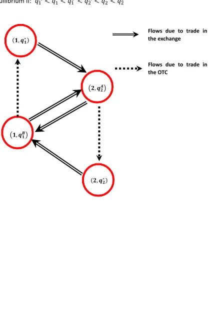
In the exchange, investors in state (1; q2), who were previously in state (2; q2) before preference shocks occur to them, are sellers and investors in state (2; q1), who were in state before they receives preference shocks, are buyers. Investors in state (i; q) with q 6=qi are searching in the OTC market to wait for the opportunity of contacting dealers and adjusting their portfolios. The pattern of ‡ows between states is depicted in Figure 1. Each circle represents a state. The dashed arrows represent ‡ows due to trade in the OTC, the double-line arrows represent ‡ows due to trade in the exchange and the solid arrows indicate ‡ows due to type changes.
We are in a position to describe the set of equations that characterize the steady-state distri-7
bution H(i; q). First, the measure of investors with preference type iis equal to i, so
n(1; q1) +n 1; qA2 +n 1; qB1 = 1; (43)
n(2; q2) +n 2; qA2 +n 2; qB1 = 2: (44)
Second, all assets are held by investors, so the market clearing condition requires
q1n(1; q1) +q2A n 1; q2A +n 2; q2A +qB1 n 1; qB1 +n 2; q1B +q2n(2; q2) =s: (45)
Third, the ‡ow of investors into each ergodic state is equal to the ‡ow out of that state. The ‡ow-balance equations are listed in the appendix and omitted here.
De…nition 2 Given A and B, the steady-state (partial) equilibrium consists of the asset price in the exchange P, intermediation fee in the OTC market fi(q; qi), the critical asset holdings
qiA; qi; qiB i=1;2, the time-invariant distribution of investors across the ergodic statesfn(i; q) : (i; q)2 g
where is given by (42), such that
fn(i; q) : (i; q)2 g satis…es (43), (44) and the ‡ow-balance equation for each ergodic state,
(41) characterizes the optimal choice for an investor in state (i; q) where i 2 f1;2g and
q 0,
qi, qiA and qiB satisfy (36), (39) and (40) respectively,
P satis…es (45),
fi(q; qi) satis…es (37).
The steady-state distribution fn(i; q) : (i; q)2 g are given by (101) (106), which are ob-tained by solving (43), (44) and all the ‡ow-balance equations. These equations have nothing to do with the utility speci…cation and the critical asset holdings.
consistent with empirical results. Note that now the transaction size is endogenously determined and varies across di¤erent trades, so we want to know whether this model can capture the fact that the trading frequency in the exchange is much higher than that in the OTC. However, we …nd the number of trades in the two markets are the same. One conjecture is that investors’ valuations are assumed to take only two values. If investors become more heterogenous in their valuations, we might have the desirable result. Third, compared with the frictionless benchmark, investors of low (high) type hold too many (few) units of asset, i.e.,q1 > qW1 ; q2 < q2W.
Under monopolistic market making, the optimal bid-ask spread is given by
A B =
r+ + (1 ) +
c
2:
This is almost the same as(28), so how the bid-ask spread is related to the underlying parameters are the same as before. It has to be admitted that this result is due to the quadratic utility speci…ed in (33). If some other speci…cations of instantaneous utility are chosen, the optimal bid-ask spread could take some other forms or the closed-form solutions are not available. It is interesting to check whether the same comparative statics results could be maintained under di¤erent utility speci…cations or not.
Equilibrium II:q1A< q1B< qA2 < qB2. Now consists of 4 states
= (1; q1); 1; q1B ; 2; q2A ;(2; q2) :
The pattern of ‡ows between states is illustrated in Figure 2. It turns out that any investor goes to trade in the exchange whenever there is a change in his preference type.
5
Conclusion
We have analyzed a model where investors can trade a long-lived asset in both exchange and OTC market. In the exchange, transactions are intermediated by market-makers who post bid-ask prices publicly. In the OTC market, dealers search for trading partners on behalf of investors. Exchange means high immediacy and high cost while OTC market corresponds to low immediacy and low cost. We show that in equilibrium investors with urgent trading needs enter the exchange while investors with medium valuations enter the OTC market. We analyze how the bid-ask spread is related to underlying parameters and specify the boundary of active trading in each market. We also conduct welfare analysis and …nd that the decentralized solution is always inferior to the socially optimal solution in terms of total welfare.
Figure 1
Equilibrium I:
𝑞
1𝐴< 𝑞
1∗< 𝑞
2𝐴< 𝑞
1𝐵< 𝑞
2∗< 𝑞
2𝐵𝟏, 𝒒
𝟏∗𝟏, 𝒒
𝟏𝑩𝟐, 𝒒
𝟏 𝑩
𝟐, 𝒒
𝟐∗Flows due to type change
Flows due to trade in
the exchange
Flows due to trade in
the OTC
𝟏, 𝒒
𝟐𝑨Figure 2
Equilibrium II:
𝑞
1𝐴< 𝑞
1∗< 𝑞
1𝐵< 𝑞
2𝐴< 𝑞
2∗< 𝑞
2𝐵𝟏, 𝒒
𝟏∗𝟏, 𝒒
𝟏𝑩𝟐, 𝒒
𝟐∗Flows due to trade in
the exchange
Flows due to trade in
the OTC
Appendices for Chapter 1
6
Appendix I
In this section, we state and prove the steady-state (partial) equilibrium given the bid and ask prices in the exchange, A and B. Proposition 1 in Section 2.2 is just a special case by taking
= 0here.
Theorem 1. Given that c A B < + ++r , the partial steady-state equilibrium given A
and B is characterized as follows. and are uniquely determined by
= ( +r) ;
(1 s)F( ) +sF( ) = 1 s:
0 and 1 are uniquely determined by
(1 s)F( 0) +sF( 1) = 1 s;
A B = 0 1+
+ +r :
Investors’ distributions are given by
n( ) =
8 > > > > > < > > > > > :
f( ) for 2[ ; 1) (1 s)+
+ f( ) for 2[ 1; ]
(1 s)f( ) for 2( ; )
(1 s)
+ f( ) for 2[ ; 0]
0 for 2 0;
; (46)
o( ) =
8 > > > > > < > > > > > :
0 for 2[ ; 1)
sf( )
+ for 2[ 1; ]
sf( ) for 2( ; )
s+
+ f( ) for 2[ ; 0]
f( ) for 2 0;
The asset prices are given by
PA =
1 +
r r
R
1 F( )d
+ +r r
R
F( )d
+r + r
R 0
[1 F( )]d
+ +r ;
A PA = 0
+ +r;
PB B = 1
+ +r;
PA PB = :
Proof of Theorem 1: The proof is organized as follows. We reformulate the value function for owners and non-owners in Step I. We make some preliminary analysis in Step II. Step III and IV determine the optimal strategy for non-owners and owners, respectively. The asset prices are derived in Step V. We show the population distribution for non-owners and owners in Step VI and solve out all cuto¤ points in Step VII.
Step I. De…ne the following three disjoint subsets of the whole range ; :
N = n 2 ; jVn( )>max
n
VbOTC( ); Vbexchange( )oo;
BOTC = n
2 ; jVbOTC( )>max
n
Vn( ); Vbexchange( )
oo
;
Bexchange = n
2 ; jVbexchange( )>max Vn( ); VbOTC( )
o
:
That is, a non-owner chooses to do nothing if his valuation is in N, to search to buy the asset in the OTC market if his valuation is in BOTC and to buy in the exchange if his valuation is in Bexchange. Note that the valuations with which a non-owner is indi¤erent between any of the two choices are not included in any of the three subsets de…ned above, so the union of the three subsets is not necessarily the whole range, i.e., N [ BOTC[ Bexchange ; . These indi¤erence valuations are in the boundary but not the interior of those subsets. Denote by@N the boundary of N, namely,
@N =n 2 ; jVn( ) = max
n
VbOTC( ); Vbexchange( )oo;
market, i.e.,
@N \@BOTC= n
2 ; jVn( ) =VbOTC( ) V
exchange
b ( )
o
:
The meaning of set @Bexchange[ @BOTC and @Bexchange[ @N can be understood in the similar way. The union of N and its boundary@N is called the closure ofN and denoted by cl(N), and the same for the other two subsets. Note that cl(N), cl(BOTC)and cl(Bexchange)are not mutually disjoint, but the union of them is exactly ; .
(3) can thus be written as
V (0; ) =
8 < :
Vn( ), if 2cl(N)
VOTC
b ( ), if 2cl(BOTC)
Vbexchange( ), if 2cl(Bexchange)
:
Similarly, we de…ne the following three disjoint subsets of the whole range ; :
H =
n
2 ; jVh( )>max
n
VsOTC( ); Vsexchange( )
oo
;
SOTC = n
2 ; jVsOTC( )>maxnVh( ); Vsexchange( )
oo
;
Sexchange = n
2 ; jVsexchange( )>max VsOTC( ); Vh( )
o
:
That is, an owner holds onto his asset if his valuation is in H, searches to sell his asset in the OTC market if his valuation is in SOTC and chooses to sell in the exchange if his valuation is in
Sexchange. Likewise, these subsets do not include the valuations with which owners are indi¤erent between any of the two choices. We de…ne the boundary and closure of each subset as above.
(7) can thus be written as
V (1; ) =
8 < :
Vh( ), if 2cl(H)
VOTC
s ( ), if 2cl(SOTC)
Vsexchange( ), if 2cl(Sexchange)
:
It should not be optimal for an owner to sell his asset in the OTC market in the …rst place and then buy back the asset, still, through search in the OTC market after he sells his asset, given no change in his valuation, otherwise he would choose to hold onto it at the very beginning. This means
Similarly, it should not be optimal for an owner to sell his asset in the exchange in the …rst place and then buy back the asset in the exchange immediately given no change in his valuation. This means
Sexchange ; ncl(Bexchange) =N [ BOTC[(@N \@BOTC): (49)
The same logic should apply to buyers in the OTC and the exchange market, so
BOTC ; nSOTC=H [ Sexchange[(@H \@Sexchange), (50)
Bexchange ; nSexchange=H [ SOTC[(@H \@SOTC). (51)
Step II. Let’s …rst argue thatSexchange\ BOTC=?. Suppose not, i.e., Sexchange\ BOTC6=?. This means that (i) the owners with valuations in this set would …rstly sell their assets in the exchange and then search to buy in the OTC afterwards, and (ii) the non-owners with valuations in this set would …rstly search to buy in the OTC and then sell in the exchange immediately after they acquire the assets. When 2 Sexchange\ BOTC, we have
VbOTC( ) =
h
Vsexchange(1; ) PA
i
+ E[V (0; 0)]
+ +r ;
Vsexchange( ) = VbOTC( ) +B;
which can be solved by
VbOTC( ) = (B PA)
+r +Vn;
Vsexchange( ) = (B PA)
+r +Vn+B:
Note that we must have VbOTC( ) > Vn if 2 Sexchange\ BOTC BOTC, so we know from above thatB > PA, which contradicts(2). Hence, we claimSexchange\ BOTC=?. It thus follows that Sexchange N according to(49) and BOTC H according to(50).
buy assets in the exchange and then search to sell them in the OTC. When 2 SOTC\ Bexchange,
VsOTC( ) =
1 + + hVbexchange( ) +PB
i
+ E[V(1; 0)]
b + +r
;
Vbexchange( ) = VsOTC( ) A;
which can be solved as
VsOTC( ) = Vh( )
(A PB)
+r ;
Vbexchange( ) = Vh( )
(A PB)
+r A:
Note that we must have VsOTC( ) > Vh( ) if 2 SOTC\ Bexchange SOTC, so we know from above that A < PB, which contradicts (2). Hence, we claim SOTC\ Bexchange =?. It thus follows that SOTC N according to(48) and Bexchange Haccording to (51).
We can use the above results to simplify equations(5);(6);(9) and (10)as follows:
VbOTC( ) = [Vh( ) PA] + E[V (0;
0)]
+ +r (due toBOTC H), (52) Vbexchange( ) = Vh( ) A (due toBexchange H), (53)
VsOTC( ) = 1 + + (Vn+PB) + E[V (1;
0)]
+ +r (due toSOTC N), (54) Vsexchange( ) = Vn+B (due toSexchange N). (55)
Step III. We now prove that the optimal strategy for a non-owner is shown in (11), i.e.,
N = [ ; );
BOTC = ( ; 0);
Bexchange = 0; :
We …rst argue that if x1 2 N, thenx 2 N for all x < x1. Suppose not, i.e., there exists x2
with x2 < x1 butx2 2 N= . Ifx22 BOTC, then
However, we know
VbOTC(x2) VbOTC(x1) =
[Vh(x2) Vh(x1)]
+ +r =
(x2 x1)
( + +r) ( +r) <0;
where the …rst equality is due to(52)and the second equality is due to(8). This contradicts(56). We then turn to assume x2 2 Bexchange, which implies
Vh(x1) A=Vbexchange(x1)< Vn< Vbexchange(x2) =Vh(x2) A:
This, again, impliesx2> x1, which contradicts our starting assumption. We thus prove the claim.
We now argue that if y12 Bexchange, theny 2 Bexchange for ally > y1. Suppose not, i.e., there
exists y2 withy2 > y1 buty2 2 B= exchange. Ify22 BOTC, thenVbexchange(y2)< VbOTC(y2)implies
Vh(y2)< A+Vn+
(A PA)
+r ;
and Vbexchange(y1)> VbOTC(y1) implies
Vh(y1)> A+Vn+
(A PA)
+r :
These two inequalities, together, imply y1 > y2, which contradicts our starting assumption. If
y2 2 N, then Vbexchange(y2)< Vnimplies
Vh(y2)< Vn+A:
and Vbexchange(y1)> Vn implies
Vh(y1)> Vn+A:
These two inequalities imply y1 > y2, which presents a contradiction again. We thus prove the
claim.
The above arguments establish the claim in the very beginning of this step. The slope of
V (0; ) in each region is given by
dV (0; )
d =
8 < :
0, if 2[ ; )
+ +r
1
+r, if 2( ; 0)
1
+r, if 2 0;
We see thatV (0; ) is piece-wise linear in . Integrating(57), we obtain
V (0; ) =
8 < :
Vn, if 2[ ; )
Vn+ + +r +r , if 2[ ; 0]
Vn+ + +r 0+r + +r0, if 2 0;
: (58)
We now derive the expression ofVn. For this, we …rst calculate E[V (0; 0)]:
E V 0; 0 = Vn+
+ +r
R 0
( )dF( )
+