2016 6th International Conference on Information Technology for Manufacturing Systems (ITMS 2016) ISBN: 978-1-60595-353-3
1. INSTRUCTIONS
Compressed Sensing (CS)[1] is an emerging developed theoretical framework for information acquisition and processing, which breaks the limitation of traditional sampling theorem. It includes three parts: sparse representation of signals, design of measurement matrix and reconstruction algorithm. Based on it, the signals can be reconstructed from fewer linear measurements by taking advantage of the sparsity or compressibility of signal itself under the proper representation.
The reconstruction algorithms take up an important role in the CS, especially in its successful and wide applications. Presently, various algorithms are proposed for CS reconstruction, which can be divided into three categories[2]: (1) the greedy pursuits, such as the matching pursuit (MP) series algorithms. (2) The convex relaxation algorithms, such as the interior-point algorithm, the gradient projection (GP) algorithm, the iterative thresholding algorithm (ITA)[3], and the fixed-point continuation (FPC) method[4]. (3) The combinatorial algorithms.
Recently, one widely applied algorithm is the iterative soft-thresholding method (IST) and its improvements, including two-step IST (TwIST)[5] and fast IST (FITS) [6]. Furthermore, a new version, the fixed point continuation (FPC) method, is given in [4] by interpreting IST as a fixed point iteration constructed from an operator splitting technique. Its field of application is wider, and it doesn't need to compute the second-order Hessian matrix, which
greatly reduces the computational complexity, hence the study of FPC method has a certain meaning and value. A fast algorithm of FPC will be proposed, which keeps the original reconstructed performance of algorithm, and then improves the speed and quality of reconstruction.
The paper is organized as follows. In Section 2, we will introduce the reconstruction model and algorithms of CS. In Section 3, we propose a fast algorithm of FPC, and give some theoretical analysis of the algorithm performance. In Section 4, we present our numerical experiments and show the convergence and high efficiency of algorithm. And in Section 5, we conclude the paper.
2 BACKGROUND
2.1 Model of CS reconstruction
Assume that x∈Rnis the K-sparse signal, and then
it can be reconstructed from relatively few incomplete measurements b= Ax for a carefully
chosen A Rm×n
∈ by solving the l0-minimization
problem
b Ax t s x
n
R x
=
∈
. . || ||
min 0 (1)
Where ||x||0 is the l0-norm with ||x||0 = {i, xi≠0}, and K≤m≤n. Unfortunately, it is not convex and the
computational complexity of optimizing is NP hard. So, it is tractable for us to solve it through the existing optimization algorithm. Then, Donoho etc.
A Fast Fixed Point Continuation Algorithm with Application to
Compressed Sensing
Qingqing Guo, Lei Li
School of Science, Nanjing University of Posts and Telecommunications, Nanjing 410023, China
ABSTRACT: Fixed point continuation (FPC) algorithm is a developed version of convex optimization algorithm, which is an important research method for reconstruction of Compressed Sensing (CS). In this paper, a fast FPC (FFPC) algorithm is proposed to accelerate the convergence speed of FPC algorithm. It is introduced into an efficient shifting step, and its current iteration is updated by using special linear combination of two previous iterations. Therefore the accuracy of each iteration is improved, and the convergence speed is accelerated. In the numerical experiments, the convergence of FFPC algorithm is proven, the convergence speed of FFPC algorithm is obviously improved compared with the standard FPC algorithm, and the reconstruction quality is better than other algorithms.
KEYWORDS: Convex optimization algorithm; Compressed sensing; Fixed point continuation algorithm
[1,7] have shown that the solution x of the problem (1) can be found by solving the basis pursuit (BP) problem, under some reasonable conditions on x and A. b Ax t s x n R x = ∈ . . || ||
min 1 (2)
Where ||⋅||1 denotes the l1 norm
with =
∑
n= i xix1 1 .
In this way, the non-convex problem is transformed into a convex one, which can be simplified to linear programming for us to solve. However, if the measurement b is blurred with noise,
then an appropriate norm of the residual Ax - b should be considered, and which norm to use depends on the nature of the noise. Such considerations yield a family of related optimization problems. And if there is Gaussian noise in b, the
l1-regularized least squares problem would be
appropriate as follow.
2 2
1 || ||
2 || ||
min x Ax b
n R x − + ∈ µ (3)
Where µ > 0. The theory for penalty functions implies that the solution (3) goes to the solution of (2) as µ goes to zero. It has been shown in [8] that (2)
is equivalent to (3) for a suitable choice of b (which is different from the b in (3)).
2.2 Fixed point continuation algorithm
Set g x( ) || ||= x 1 and 2
2
( ) || || /2
f x = Ax−b , then objective function (3) can be expressed as
min ( )F x =g x( )+µf x( ).
It is well known that minimizing a convex function F(x) is equivalent to finding a zero of the subdiffenrential ∂F(x)[9], i.e., finding x such that
) ( ) (
0∈∂F x =T x , where T is a maximal monotone
operator. One can split F(x)into a sum of two convex functions, F=F1+F2 , based on the operator splitting, then it implies that the decomposition of Texits, which is the sum of two
maximal monotone operators, T=T1+T2. Then, for some
τ
>0:x T I T I x x T I x T I x T x x T x x T ) ( ) ( ) ( ) ( )) ( ( )) ( ( 0 ) ( 0 2 1 1 2 1 2 1 τ τ τ τ τ τ − + = ⇔ − ∈ + ⇔ − − + ∈ ⇔ ∈ − (4)
Where, the equation (4) finds a zero of Tby FB
splitting algorithm, otherwise, the equation leads to a minimal solution of F(x):
n n x T I T I
x ( ) ( 2)
1 1
1= +τ − −τ +
(5)
Which is a fixed point (FP) algorithm. For the minimization problem, T2(x)=
µ
∇f(x) ,1 1(x) ||x||
T =∂ , and (I+τT1)−1 is shrinkage.
Proposition 1. Supposing that X*is the set of
optimal solution of (3), for some scalar
τ
>0 , if **
X
x ∈ , x*satisfies the following equation, by:
} 0 , | ) ( max{| )) (
sgn( * * * *
*
µ τ τ
τ∇ − ∇ −
−
= x f x x f x
x o
Hence the FP equation is a composition of two mapppings: svand hτ, defined as:
( ) ( ) ( )
( ) sgn( ) max{| | , 0}.
v
h I f
s v
τ ⋅ = ⋅ − ∇τ ⋅
⋅ = ⋅ o ⋅ − (6)
Where µ,τ >0, v=τ/µ, and using a constant
parameter ) / 2 , 0 ( λmax
τ∈ with λmax =max{∇2f(x)} to ensure
that ( )h ⋅ is non-expansive.
In addition, considering continuation of FP algorithm, the paper [9] has proposed a continuation
strategy for µ defined by an increasing sequence {µi}. When a new problem, associated with
1
+
i µ , is
to be solved, the approximate solution for the current
i
µ problem is used as the starting point. This
formal statement is called fixed point continuation (FPC) method.
2.3 Properties of FPC algorithm
Define 1. The object problem (3) has an optimal
solution set X ≠∅, and there exists a set
n R x
x
x − ≤ ⊂
=
Ω { : * ρ} (7)
For some *
x ∈X and ρ >0.
Lemma 1. The operator (⋅)
v
s is non-expansive,
i.e. for any n R x
x1, 2∈ ,
|| || || ) ( ) (
||sv x1 −sv x2 ≤ x1−x2 (8)
Lemma 2. Assume
τ
∈(0,2/λ
ˆmax), and under define 1, the operatorhτ(⋅)is non-expansive in Ω, i.e., for any x,x'∈Ω,|| ' || || ) ' ( ) (
||hτ x −hτ x ≤ x−x (9)
Moreover, g(x)=g(x')whenever equality holds in the (9).
Theorem 1. Under lemma 1 and 2, given a
special τ, and a fixed point *
x , the sequence
{ || *||
x
xn− } generated by FPC iteration is
monotonically non-increasing, *
*
1 x x x
xn+ − ≤ n− (10) Proof: * * 1 * * || || || ( ) ( ) || || ( ) ( ) || || ||
n v n v
n
n
x x s h x s h x
h x h x
x x τ τ τ τ + − = − ≤ − ≤ −
Above, the inequality is proven straightforwardly.
Lemma 3. For x*∈Ω , if
* *
*) ( ) (
)
(x s h x s h x x x x
h
is a fixed point (and therefore a solution of (3)), that is, x=svhτ(x).
Theorem 2. The sequence {xn} generated by the
FPC iteration applied to the problem (3) from any starting point x0∈Ω converges to some
*
x ∈X ∩ Ω.
Proof:
Depend on the lemmas mentioned above, to prove the convergence of {xn}, it needs three steps.
First, show the sequence {xn} has a limit point.
Since shτ(⋅)
v is non-expansive, { xn } lies in a
compact subset of Ω, so it must have a limit point,
that is, j
n
j x
x
∞ →
=lim .
Second, there exists a fixed point. Because of any given fixed point *
x , the sequence {||xn−x*||} is
monotonically non-increasing, it has a limit that can be written as
* *
lim xn x x x n
− = −
∞
→ (11)
Where x can be any limit point of {xn}.
Next, prove the uniqueness of the solution. We know, all the limit points must have an equal distance to any given fixed point * *
X
x ∈ .
Based on the continuity of shτ(⋅)
v , the image of x is also a limit point of { xn }, where
j
j j n
n v j
vh x sh x x
s
∞ → ∞
→
= =lim ( ) lim )
( τ
τ . Therefore, from
(11) we have ( ) ( *) *
x x x h s x h
sv τ − v τ = − , then
apply the lemma 3 to x and establish the
optimality of x . By setting x*=x∈X*in (11), we
can obtain the convergence of {xn} to its unique
limit point x:lim − =0
∞ → xn x
n .
Finally, the proof of theorem is end, the more detail process can be seen [9].
3 PROPOSED ALGORTIHM
3.1 Fast fixed-point continuation algorithm
The FPC algorithm has two phases. One is gradient descent step with some appropriate constant, another is shrinkage threshold. The advantage of FPC algorithm is in its simplicity. However, the algorithm has also been recognized as a slow method, since its computational efforts. As expected, a fast FPC algorithm is required to be proposed. There are many modifications proposed recently, such as two-step version of fixed point continuation method, and adaptive fixed-point iterative shrinkage thresholding algorithm etc.[10]. In this paper, we focus in the design of shifting step in iteration to improve the convergence and efficiency of FPC algorithm.
For achieving faster convergence of (F(xn))n∈N
than the ISTA algorithm, FISTA utilizes a shifting
step from xn to yn. Similarly, we will introduce a
shifting step to the FPC algorithm, based on the precious two iterative steps. So an improved algorithm, FFPC algorithm, is proposed. And It is believed that the new algorithm can obtain the accelerating convergence, and is more aggressive. In addition, in view of one more step approximation at each iteration, the improved algorithm will obtain a more precise solution. The FFPC algorithm defines a sequence xn by:
1
1
( ( )),
1
( ) , .
n v n n
n
n n n n n n
n
x s y f y
t
y x x x with
t τ
α α
−
+
= − ∇
−
= + − = (12)
Since the efficient coefficient of the shifting step depends on the sequence(αn), the choice of ( )
n t is
the critical point of the improved algorithm. For FIST algorithm, a special sequence, t1=1 and
N n t
tn+ = + + n , ∀ ∈
2 4 1
1 2
1 , is selected, which is
proven to be significantly better on the global rate of convergence than the standard IST algorithm, both theoretically and practically[6]. What’s more, the paper [11] has presented some different sequences,
and analyzed the convergence of new algorithm using various coefficients for shifting step. One type is =1+ + , ∀n∈N witha≥2
a n a
tn , which
accelerates the convergence of ISTA algorithm at some extent.
Therefore, making full use of these sequences, several improved algorithms can be proposed. Since these choices can optimize the IST algorithm, we believe that they can improve the FPC algorithm. Furthermore, these variants can ensure the convergence, as well as the efficiency and accuracy. In addition, the performance of the improved algorithms will be illustrated by the experimental result.
3.2 Enhanced FFPC algorithm
In the FPC method above, the parameter τ in process is fixed so that the fixed point iteration is a contraction at every iteration. Since a bad value of τ usually slows down the rate of convergence, the literature [11] choose τ dynamically to improve the
performance of shrinkage. It has provideda strategy, which was based on the Barzilai–Borwein (BB) method, for choosing the parameter τk . such as following:
2 1
1 1
( ) ( )
k k
x x
k xk xk T fk fk
τ
− − =
− −
− ∇ −∇ (13)
Since, τ is not chosen to ensure contraction, so a backtracking line search is necessary to guarantee global convergence, a nonmonotone line search (NMLS) method was used with Armijo-like condition[9]. And FFPC algorithm in our paper is a combination of two methods mentioned above (BB steps and NMLS method). This algorithm is reported to be faster than the benchmark. Given the algorithm of FFPC.
Algorithm 1: FFPC Algorithm
(1).Input: signal data N i i x} 1
{ = , max number of
iterations mxitr, and sparsity threshold Th, and
sequence{µi}.
(2).Initialization: sensing matrix A, measurement
noise sig initial observationx0, and initial τ0 and
0
µ .
(3).While
µ
=µ
1,µ
2,...,µ
L do the following steps: A. Check for 0 solution,B. Main loop: for k=1:mxitr, repeat the following steps until convergence or overstep.
a. Set v=τk/µ for this round; b. Take fixed point step: calculateyk =xk−1−τ⋅xk−1,
calculate =sgn( ) max{| |−ν,0}
k k
k y y
x o .
C. Non-monotone line search, get BB step, and update current iteration xk.
D. Update xk =zk−αk⋅(zk −zk−1) E. Select ,tk and compute αk
(4).Output: reconstruction *
x , time(T), and PSNR
4 NUMERICAL EXPERIMENTS
In this section the simulations based on MATLAB7.0 is carried out using a PC with CPU of Intel(R) i3 2.53 GHz and 2GB RAM.
4.1 Convergence examples
In this experiment, we evaluate the suitability of various improvements of FPC algorithm for sparse reconstruction. Given the dimension of the signal
8 2
=
n , the number of observation m=delta*n, and the number of nonzeros k=rho*n. We do a lot of tests with delta ranging from 0.3 to 0.7 and rho ranging from 0.1 to 0.5. After analyzing the results, we set delta=0.3 and rho=0.2 in terminal test. In addition, a stopping rule (1E-4), based on the relative error between adjacent iterations, is designed. And we choose two types of the sequences
N n n t )∈
( . Given as following:
Sequence1:t = andtn+ = + + tn ,∀n∈N
2 4 1 1 1
2
1
1 ;
Sequence2: tn 1 a n, n N a
+ +
= ∀ ∈ , with a=2,3,4.
Simply, the improved algorithms respectively are called FFPC, FFPC1 (a=2), FFPC2 (a=3), FFPC3 (a=4).
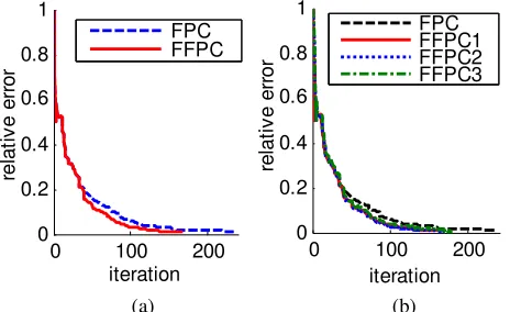
We analyze the convergence of the improved algorithms by the relative error between original and reconstructed value. If the error sequence converges to zero along with the growth iteration, the convergence of methods is thought confirmed and well-deserved. The relative error formula is as following:
2 2 2 2
s
s
x x
rerr x
−
= (14)
Where x denotes reconstructed value, and xsis
original signal.
When the sampling rate is 0.3 and sparse degree is 0.2, the experimental curves are as follow Figure 1. As we can see, the curves using improved algorithms are closer to zero with fewer iterations, which proves that the improved algorithms are convergent and converge to a optimal solution. Furthermore, the feasibility and robustness of the algorithm are verified.
4.2 Reconstruction for video frame
In this section, we select a video frame of foreman as the test objection. So the dimension of the signal is M×N=352×288, then given the number of observation m=delta*M with delta=0.3,0.5,and 0.7. On the other hand, we generate a sensing matrix
A with measurement matrix Φ and sparse basis
matrix Ψ. In general, we randomly select m rows
from a random Gaussian matrix to generate measurement matrix, and obtain a sparse signal based on orthonormal matrix (such as discrete cosine transform (DCT) matrix) in the compressed sensing reconstruction process. And, in view of the actual, the original signal is blurred by a zero-mean white Gaussian noise with standard deviation 1E-3. In
0 100 200
0 0.2 0.4 0.6 0.8 1
iteration
re
la
ti
v
e
e
rr
o
r
FPC FFPC
0 100 200
0 0.2 0.4 0.6 0.8 1
iteration
re
la
ti
v
e
e
rr
o
r
FPC FFPC1 FFPC2 FFPC3
(a) (b)
[image:4.612.317.549.534.676.2]In order to demonstrate the effectiveness of the various improvements of FPC algorithm, we reconstruct the video frame respectively using the standard FPC, FFPC, and FIST algorithms. After simulating, we compare the numerical results and analyze the performance of them.
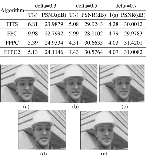
[image:5.612.55.298.304.557.2]In the Table 1, we list two symbols represented the effectiveness of reconstruction, reconstructed time and PSNR. As we can see, the reconstructed time of FFPC algorithms is shorter than the original FPC and FITS algorithms. It shows that the convergence speed of variants is faster than the others. At the same time, it is interesting to find that the FFPC algorithms have a better reconstructed quality from the results. Based on conclusions above, FFPC algorithms not only accelerate the speed of convergence, but also improve the quality of reconstruction. Therefore, it is an efficient and fast algorithm. The corresponding reconstruction frame depicted in figure 2.
Table 1. Reconstructed time and PSNR of video frame.
Algorithm delta=0.3 delta=0.5 delta=0.7 T(s) PSNR(dB) T(s) PSNR(dB) T(s) PSNR(dB) FITS 6.81 23.9879 5.08 29.0243 4.28 30.0012
FPC 9.98 22.7992 5.99 28.0102 4.79 29.9783 FFPC 5.39 24.9334 4.51 30.6635 4.03 31.4201 FFPC2 5.13 24.1146 4.43 30.5764 4.07 31.0082
(a) (b) (c)
(d) (e)
Figure 2. Reconstructed video frame based on different algorithms with delta=0.5 (where, (a) original video frame, (b),(c),(d) and (e) are respectively reconstruction image based on FIST, FPC, FFPC and FFPC2 algorithm).
5 CONCLUSION
In this paper, we propose a fast fixed point continuation (FFPC) algorithm family to accelerate the convergence speed of original FPC algorithm. The iteration of improved algorithm depends not only on the new iteration but also on the previous two iterations. In our numerical experiments, the convergence of FFPC algorithm is proved, and its speed is faster than the original. In addition, the
results about reconstruction of video frame based on Compressed Sensing (CS) show that FFPC algorithms are feasible and efficient, and are improved significantly. In general, the FFPC algorithm is a fast and efficient version.
6. ACKNOWLEDGEMEN
This work was supported by National Natural Science Foundation of China (Grant No.61501251, 61373137, 61071167) , Sponsored by NUPTSF (Grant No.NY214191) and university graduate student research innovation project of Jiangsu province in 2015(KYZZ15_0236). We would like to thank anyone who is helpful for us to complete this paper.
REFERENCES
[1] Donoho, D. L. 2006. Compressed sensing. IEEE Trans.inform.theory, 52(4), 1289 - 1306.
[2] Needell, D., & Tropp, J. A. 2009. Cosamp: iterative signal recovery from incomplete and inaccurate samples. Applied & Computational Harmonic Analysis, 26(3), 301-321. [3] Blumensath, T., & Davies, M. E. 2008. Iterative
thresholding for sparse approximations. Journal of Fourier Analysis & Applications, 14(5-6), 629-654.
[4] Hale, E. T., Yin, W., & Zhang, Y. 2008. Fixed-point continuation for $\ell_1$-minimization: methodology and convergence. Siam Journal on Optimization, 19(3), 1107-1130.
[5] Bioucas-Dias, J. M., & Figueiredo, M. A. T. 2007. A new twist: two-step iterative shrinkage/thresholding algorithms for image restoration. IEEE Transactions on Image Processing A Publication of the IEEE Signal Processing Society, 16(12), 2992-3004.
[6] Beck, A., & Teboulle, M. 2009. A fast iterative shrinkage-thresholding algorithm for linear inverse problems. Siam Journal on Imaging Sciences, 2(1), 183-202.
[7] Candes, E. J., & Romberg, J. 2006. Quantitative robust uncertainty principles and optimally sparse decompositions. Foundations of Computational Mathematics, 6(2), 227-254. [8] Yin, W., Osher, S., Goldfarb, D., & Darbon, J. 2008.
Bregman iterative algorithms for l1-minimization with applications to compressed sensing. siam j imaging sci 1:143-168. Siam Journal on Imaging Sciences, 1(1), 143--168.
[9] Hale, E. T., Yin, W., & Zhang, Y. 2007. A fixed-point continuation method for '1-regularized minimization with applications to compressed sensing. Caam Tr.
[10] Jiang, J., Zhang, H., & Yu, S. 2011. A Novel Monotonic Fixed-Point Algorithm for l 1 -Regularized Least Square Vector and Matrix Problem. High Performance Networking, Computing, and Communication Systems. Springer Berlin Heidelberg.
[11] Chambolle, A., & Dossal, C. (2015). On the convergence of the iterates of the “fast iterative shrinkage/thresholding algorithm”. Journal of Optimization Theory & Applications, 166, 1-15.
[12] Wen, Z., Yin, W., Goldfarb, D., & Zhang, Y. (2010). A fast algorithm for sparse reconstruction based on shrinkage, subspace optimization, and continuation. Siam Journal on Scientific Computing, 32(4), 1832-1857.
[image:5.612.56.297.305.560.2]