Seeking the Optimal Solution to Bilevel Linear Programming by Dual Problem

2016 International Conference on Mathematical, Computational and Statistical Sciences and Engineering (MCSSE 2016) ISBN: 978-1-60595-396-0

Seeking the Optimal Solution to Bilevel Linear

Programming by Dual Problem

Yi-fan ZHAO

, Shen-hua YANG

, Yong-feng SUO

and Li-yang ZHAO

1_{College of Navigation, Jimei University, Xiamen 361000, China;}

2_{College of Science, Chongqing Normal University, Chongqing 404100, China}

*Corresponding author

Keywords: Bilevel linear programming, Penalization function, Dual problem, Duality gap, Globally optimal solution.

Abstract. In view of the linear feature of the upper-level and lower-level objective function of the bilevel programming as well as its constraint conditions, this paper presented a global optimization method. Replaced low-level sub-problem of the bilevel linear programming problem with dual problem, and then added the duality gap of the lower-level problem to the upper-level objective function, as a penalty function, and solved single level mathematical programming problem as an alternative to seek the optimal solution of the original problem. Numerical experiments show that the proposed algorithm is effective and feasible. This paper avoided the complexity with solving the dual problem's constraint domain pole, thus saved computing time and energy.

Introduction

Consider the bilevel linear programming problem below.

0

. .

) , ( min ) b (

, 0

) , ( min ) a ( LBP) (

2 2

Y

1 1

X



 

 



 

 

y

b By Ax t s

y d x c y x f

solution the

is y x

y d x c y x F

T T

y

T T

x

(1)

where xXRn,yYRm are the decision variables, F:XYR, f :XYR are linear

functions, 1 , 2 Rn

T T

c

c , 1 , 2 Rm

T T

d

d , bRp, A,B are respectively the coefficient matrices of constraint function.

As to bilevel programming, the parameters of its lower-level objective function and constraint conditions always use the upper-level decision variables as parameters; while the optimal value and solution of the upper objective function are influenced by the optimal solution of the lower-level__Reference[1]. After performing a study on a bilevel linear programming with its upper-level having no constraint conditions and the lower-level having a unique optimal solution, Candler and Townsley discovered an interesting feature: supposing the bilevel linear programming has limited optimal solutions, there is at least one pole, being the optimal solution of the problem, among the poles of the lower constraint domain__Reference [2]. Then, Bard on the premise that the lower-level constraint domain is bounded; it is proved that this is a common feature of all bilevel linear programming__Reference [3].

added the lower-level duality gap as the penalty function to the target function of the upper-level problem, then solved single level mathematical programming problem first in order to get the optimal solution of the original problem. However, in the algorithm mentioned in the literature [5], the first step is to calculate the pole of the dual problem’s constrained domain; this undoubtedly increased the computational complexity. Difference between the realization of the algorithms in this paper and that in the literature [5] lies in the fact that for the method in this paper it is unnecessary to seek the pole of the dual problem’s constraint domain; we can directly solve a single-level mathematical programming problem with a penalty function and get the optimal solution of the original problem. The numerical experiments show that the algorithm is effective.

Theoretically Analysis

If the constraint domain of question(1) is S { ( , ) :x y x X,y Y,Ax By b x y, , 0} 

      , for each given the top decision variable x , the feasible set of low-level problem is

S( ) {x y Y,Ax By b ,y 0}



     .

Definition 1 For any given the upper decision variables x, the rational reaction set of low-level

problem is P( ) {x y Y : y ar g mi n{ ( , ) ,f x y y S( ) } }x



   

Definition 2 IR{(x,y):(x,y)S,yP(x)} named feasible setof question 1__Reference [6]. Definition 3 If exist (x*,y*)IR, for any (x,y)IR, F(x,y)F(x,y) constant established, then we called (x,y) the globally optimal solution of question (1), referred to as optimal solution__Reference [7].

We could make two necessary hypotheses for guarantee question (1) have optimal solution, Hypothesis A Sis compact spaces no empty;

Hypothesis B Feasible setIR __Reference [8].

When the upper-level given any xS , the optimal solution of (b) is independent of c2T, the lower-level programming (b) of question (1) is equivalent to the programming problem listed below:

0

. .

) , (

min ₂

  



y

Ax b By t s

y d y x

f T

y

(2)

The dual problem of question (2) can be expressed as

0

. .

) (

) , ( min

2   

 

u

d u B t s

u b Ax x u Z

T

T

y

(3)

where, p R 

u , the feasible region of question is： U{uRp:BTud₂,u0}.

For any fixed xS, hypothesize y and u were the feasible region of question(2) and question(3)

respectively, according to the property of duality theory, the d2Ty(Axb)Tu is constant established.

Set h(x,y,u)d2Ty(Axb)Tu, then we called h(x,y,u) is the duality gap of the lower level programming problem.

Lemma 1. Hypothesize (x,y)S, if (x,y)IR, if and only if dual problem exist uU as well as, then the equality h(x,y,u)0 is constant established. __Reference [4]

U S, ) (

0 ) (

. .

) , ( min

2

1 1 ,

,



  

 

u x,y

u b Ax y d t s

y d x c y x F

T T

T T

u y x

(4)

Theorem 1 If the optimal solution of question(1) is (x₀,y₀), if and only if exist u₀U, (x₀,y₀,u₀) can be the optimal solution of question(4) .

Proof： Necessity. Cause (x0,y0) is the optimal solution of question(1), then for the x0 given by

upper problem, y₀ the optimal solution of lower problem. So (x0,y0)S , and (x0,y0)IR .

Following the Lemma 1, exist u₀U, make h(x₀,y₀,u₀)0, we get (x₀,y₀,u₀) is the optimal solution of question(4) .

Assuming (x₀,y₀,u₀) is not the optimal solution of question(4), then there is a feasible solution

) , ,

(x1 y1 u1 to satisfy F(x1,y1)F(x0,y0),h(x1,y1,u1)0,(x1,y1)∈ S,u1U.

According to the Lemma 1, exist (x₁,y₁)IR, we can obtain (x₀,y₀) isn't the optimal solution of

question(1) from F(x₁,y₁)F(x₀,y₀) , that’s in conflict with the condition that (x₀,y₀) is the optimal solution of question(1).

Sufficiency. Because (x₀,y₀,u₀) is the optimal solution of question(4), then

0 ) , ,

(x₀ y₀ u₀ 

h ,(x₀,y₀)S,u₀U, following the Lemma 1,(x₀,y₀)IR, that is the (x0,y0) is the

optimal solution of question(1).

Exist (x₁,y₁)IR, if we hypothesize (x₀,y₀) is not the optimal solution of question(1), that is for

the x1,y1 given by upper-level problem are the optimal solutions of lower-level problem, there is )

, ( ) ,

(x1 y1 F x0 y0

F  , Following the (x1,y1)IR and Lemma 1, exist u1U , there is 0

) , ,

(x₁ y₁ u₁ 

h , then (x1,y1,u1) is the optimal solution of question(4), we can draw from

) , ( ) ,

(x₁ y₁ F x₀ y₀

F  that (x₀,y₀,u₀) isn't the optimal solution of question(4), that’s in conflict with

the condition that (x₀,y₀,u₀) is the optimal solution of question(4). So the Theorem 1 was proved to be true.

In problem (4), except the linear constraint condition, still has a non-linear equality constraint, that increases the difficulty to solve the problem,then we using concept of penalty function, transform solving the problem(4) into solving the problem below

0

≥

, 0

≥

, 0

≥

≥

≤

+ . .

) ) (

( + ) , ( = ) , , (

min ₂

, ,

u y x

d u B

b By Ax t s

u b Ax y d M y x F u y x g

T

T T

u y x

(5)

where, M is any penalty factor that greater than zero, M(d₂Ty(Axb)Tu)0 is punishing item of question (5). Following the introduction of penalty function from literature[7], the following theorem is established.

Theorem 2 Exist a positive numberM₁ if question(1) have optimal solution, when MM₁, question(1) and question(5) have same optimal solution.

Descriptions of Algorithms

According to the above theory, the algorithm can be described as follows: Step 1 Given initial conditions M 1,  10, k 1, turn to step 2;

Step 2 Seeking the optimal solution of question (5) by non-linear technology, denoted by )

, ,

Step 3 Stop calculation if h(x_k,y_k,u_k)0, output the optimal solution (xk,yk) of question(1),

otherwise, turn to step 4;

Step 4 Let M M , turn step 2.

Numerical Experiment

The lower-level dual problem’s constraint domain is

0 2 5 . 0 5 . 0 -1 2 -1 3 2 1 3 2 1 3 2 1 3 2 1          u u u u u u u u u u u u ， ，

Just need to solve the optimal solution of following questions

0 , , , , , , , 2 5 . 0 5 . 0 1 2 1 1 5 . 0 -2 2 1 5 . 0 -2 -2 1 . . ) ) ( ( ) , , ( min 3 2 1 3 2 1 2 1 3 2 1 3 2 1 3 2 1 3 2 1 2 3 2 1 1 3 2 1 2 1 1                    u u u y y y x x u u u u u u u u u y y y x y y y x y y y t s u b Ax y d M y d x c u y x

g T T T T

In the first iteration, let M=1， 10, solving the optimal solution and the optimal value in the constraint domain of the objective function, as shown in table 1 below.

Table 1. Optimal solution and optimal value of the first iteration and the duality gap.

In Table 1, the target function g(x,y,u)’s optimal value is 53 . At this time, the optimal solution is (0,0,1.5,1.5,1,0,0,0), and the value of its corresponding duality gap h(x,y,u) is 5,50, perform the second iteration for M M .

Perform the second iteration, M M 10. Seek the optimal solution and the optimal value of the objective function g(x,y,u) in the constraint domain as shown in the Table 2 below:

1

x x₂ y₁ y₂ y3 u1 u2 u3

Optimal

Solution 0.0000 0.0000 1.5000 1.5000 1.0000 0.0000 0.0000 0.0000

) , , (x y u g

-53.0000

) , , (x y u h

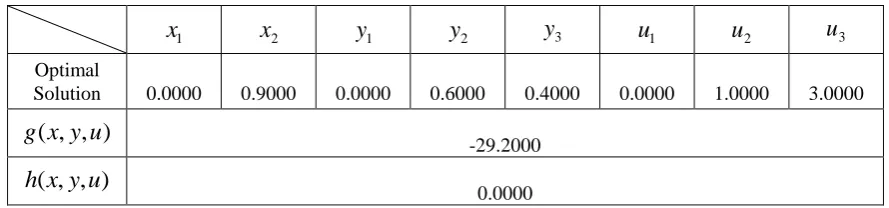
Table 2. Optimal solution and optimal value of the second iteration and the duality gap.

In Table 2, the target function g(x,y,u)’s optimal value is -29.2. At this time, the optimal solution

is (0,0.9,0,0.6,0.4,0,1,3), and the value of its corresponding duality gap h(x,y,u) is 0, and optimal solution of the problem is x(0,0.9) and y(0,0.6,0.4). This is consistent with the results in literature [5] and proves that the algorithm is feasible.

Summary

It is necessary to seek the pole of the dual problem’s constraint domain for the algorithm in literature [5]. This paper avoided the complexity with solving the dual problem’s constraint domain pole, thus saved computing time and energy. Numerical experiments showed that the algorithm is effective, feasible and of significant value for reference and application. But there is limitation with the solution in this paper. It is necessary to carry on further research on how to use a more effective method to turn lower-level constraint condition into more general non-linear constraint function and simplify the structure of the penalty function.

Acknowledgement

This research was supported by the National Natural Science Foundation of China (51579114); supported by Fujian Provincial Natural Science Foundation of China (2015J05103); supported by the project of New Century Excellent Talents of Colleges and Universities of Fujian Province (JA12181).

References

[1] W.F. Bialas, M.H. Karwan. Two-level linear programming, Managenment Science, 1984, 30 (8):1004-1020.

[2] W. Candler, R. Townsley. A linear two-level programming problem, Computers and Operations Research, 1982, 9(1):59-76.

[3] J.F. Bard, Practical bi-level optimization: algorithms and applications. Boston: Kluwer Academic Publishers, 1998.

[4] X.M. Wei, M.X. Zhao and Z.J. Zhang, A global optimization method for bilevel linear programming, J. Journal of Shandong University of Science and Technology (Natural Science), 2009, 28(1):99-102.

[5] M.X. Zhao, Z.Y. Gao, A global optimization method for solving bilevel linear programming with penalty function, Operations research and management science, 2005,14(4):25-39.

[6] C.Y. Hu, Bilevel linear programming theory and its application in management, Intellectual property press, BeiJing, 2012, 34-36.

[7] Luenberger D G. Linear and nonlinear programming, Addison-Wesley, 1984.

[8] Y. Zheng, Z.P. Wan, Global optimization method for nonlinear bilevel programming problem, Journal of Systems Science and Mathematical, 2012, 32(5):513-521.

1

x x₂ y₁ y₂ y3 u1 u2 u3

Optimal

Solution 0.0000 0.9000 0.0000 0.6000 0.4000 0.0000 1.0000 3.0000

) , , (x y u g

-29.2000

) , , (x y u h