Performance Optimization and Parallelization of a Parabolic Equation Solver in Computational Ocean Acoustics on Modern Many core Computer

2017 International Conference on Computer Science and Application Engineering (CSAE 2017) ISBN: 978-1-60595-505-6

Performance Optimization and Parallelization of a Parabolic

Equation Solver in Computational Ocean Acoustics on Modern

Many-core Computer

Min Xu1, Yongxian Wang1*, Anthony Theodore Chronopoulos2 and Hao Yue1 1

Academy of Marine Science and Engineering,National University of Defense Technology, 410073 Changsha, China

2

University of Texas at San Antonio, San Antonio, 78249 TX, USA.

ABSTRACT

As one of open-source codes widely used in computational ocean acoustics, FOR3D can provide a very good estimate for underwater acoustic propagation. In this paper, we propose a performance optimization and parallelization to speed up the running of FOR3D. We utilized a variety of methods to enhance the entire performance, such as using a multi-threaded programming model to exploit the potential capability of the many-core node of high-performance computing (HPC) system, tuning compile options, using efficient tuned mathematical library and utilizing vectorization optimization instruction. In addition, we extended the application from single-frequency calculation to multi-frequency calculation successfully by using OpenMP+MPI hybrid programming techniques on the mainstream HPC platform. A detailed performance evaluation was performed and the results showed that the proposed parallelization obtained good accelerated effect of 25.77× when testing a typical three-dimensional medium-sized case on Tianhe-2 supercomputer. It also showed that the tuned parallel version has a weak-scalability. The speed of calculation of underwater sound field can be greatly improved by the strategy mentioned in this paper. The method used in this paper is not only applicable to other similar computing models in computational ocean acoustics but also a guideline of performance enhancement for scientific and engineering application running on modern many-core-computing platform.

INTRODUCTION

Sound is the only energy form that can transmit in long distance in seawater medium. It is the most effective method of target detection and information transmission underwater[1]. Using a three-dimensional numerical model it is difficult to provide real-time acoustic field data for sonar equipment and other applications[2].Therefore, efficient large-scale parallel computing based on the latest high-performance computing platform can solve this problem.

use of the current many-core computing power. Considering these problems, this paper proposes a parallelization and optimization combining the characteristics of architecture and application program to implement the efficient simulation of real three-dimensional underwater acoustic propagation problem on Tianhe-2 supercomputer.

NUMERICAL UNDERWATER ACOUSTIC MODEL

The Parabolic Equation method (PE) is a numerical model in underwater acoustics[4]. In this paper, we use FOR3D which is a representative application program of PE to obtain a parallel algorithm program for three-dimensional underwater acoustic propagation. FOR3D used in this article can be downloaded from the Online Marine Acoustic Library (http://oalib.hlsresearch.com). The entire acoustic field is shown in Figure 1.

Figure 1. The 3D view of one sector of acoustic field.

Mathematical Process of FOR3D

The starting point of parabolic Eq. (1) is the three-dimensional Helmholtz equation in cylindrical coordinates system (𝑟, 𝜃, 𝑧) as shown in Eq. (1):

𝜕2𝑝 𝜕𝑟2+

1 𝑟

𝜕𝑝 𝜕𝑟+

1 𝑟2

𝜕2𝑝 𝜕𝜃2+

𝜕2𝑝

𝜕𝑧2+ 𝑘02𝑛2𝑝 = 0 (1)

where 𝑟, 𝜃, 𝑧 denote range, azimuth and depth respectively, 𝑝 = 𝑝(𝑟, 𝜃, 𝑧) denotes the pressure，𝑛 = 𝑛(𝑟, 𝑧)is the index of refraction and 𝑘₀ = 𝑘₀(𝜔)is the wavenumber.

By using Tappert's parabolic decomposition technique[5], let𝑝(𝑟, θ, 𝑧) = 𝑢(𝑟, θ, 𝑧)𝑤(𝑟), where 𝑤(𝑟) is the Hankel function. Eq. (1) can further be expressed in terms of 𝑢 instead of 𝑝 as shown in Eq. (2) under the “wide angle assumption”[6].

𝜕2𝑢

𝜕𝑟2+ 2i𝑘0

𝜕𝑢 𝜕𝑟+

𝜕2𝑢 𝜕𝑧2+

1 𝑟2

𝜕2𝑢 𝜕𝜃2+ 𝑘0

2_(𝑛2_{(𝑟, 𝜃, 𝑧) − 1)𝑢 = 0 (2)}

By using theoperator splitting and operator approximation technique and after a series of complicated calculations (see [7]), we obtain Eq. (3) finally

𝜕

𝜕𝑟𝑢 = (−i𝑘0+ i𝑘0[(1 + 1 2𝑥 −

1 8𝑥

2_{) +}1

where 𝑥 = 𝑘₀2(𝑛2_{(𝑟, 𝜃, 𝑧) − 1) +} 1 𝑘02

𝜕2

𝜕𝑧2 and 𝑦 =

1 (𝑘0𝑟)2

𝜕2

𝜕𝜃2 are two differential

operators[7].

To solve Eq. (3) numerically, a finite difference method is applied to discretize it in time and space. This results in an iteration-style of range advancing is formed as

[1 + (1

4− 𝛿

4) 𝑋] [1 −

𝛿 4𝑌] 𝑢

𝑗+1_{= [1 + (}1

4+ 𝛿

4) 𝑋] [1 +

𝛿 4𝑌] 𝑢

𝑗 _{= 𝑅𝐻𝑆 (4)}

where δ = 𝑖𝑘0Δ𝑟, 𝑋(and 𝑌) is the difference version (operator) with respect with differential operator 𝑥 (and 𝑦). Superscript 𝑗 and 𝑗 + 1 indicate the current step and next step of range advancing respectively. To solve Eq. (4), the following two-step marching process is used: (a) Compute right-hand side (𝑅𝐻𝑆) of Eq. (4) and obtain 𝑣𝑗+1 by solving Eq. (5). (b) Solve Eq. (6) and get the unknown 𝑢.

[1 + (1

4− 𝛿 4) 𝑥] 𝑣

𝑗+1 _{= 𝑅𝐻𝑆 (5)}

[1 −𝛿

4𝑦] 𝑢

𝑗+1 _{= 𝑣}𝑗+1 ₍₆₎

The distinct advantage of this two-step procedure is that only two tri-diagonal systems need to be solved for each step marched forward in the range. Consequently, less memory and fewer computations are required. Noticing that a central difference scheme introduced in operator 𝑋 and 𝑌 will produce a tri-diagonal linear system for both Eq. (5) and Eq. (6). Without loss of generality, we denote the discretized form of both tri-diagonal systems as follows

𝐴𝑗+1_𝑣 𝑚,𝑙 𝑗+1

= 𝑅𝐻𝑆 (7)

𝐵𝑗+1𝑢_𝑚,𝑙𝑗+1 = 𝑣_𝑚,𝑙𝑗+1 (8)

where subscripts 𝑙, 𝑚 denote the index of grid in depth (𝑧) and azimuth (𝜃) direction respectively. Superscript 𝑗 denotes the index of the grid in the range direction and the grid is shown in Figure 1.

Code and Algorithm of FOR3D

The main program of FOR3D consists of a series of subroutines. The main program contains the main loop to performthe calculation of the propulsive process by calling different subroutines to perform a variety of tasks as shown in Figure 2.

Figure 2. Algorithm of the parabolic-equation model used in FOR3D. 1 for each frequency ω of wideband signals

2 Initialization from the configurations of sound sources, receivers and sound speed profiles

3 set current range r = 0 4 while r <max_range 5 r = r + Δr

6 boundary condition

7 update matrix A and B in equation (7) and (8) 8 compute RHS in equation (4)

9 update unknown u by a tri-diagonal linear solver (two-step subroutine) 10 update pressure p = u * Hankel function

11 end while

12 next frequency

OPTIMIZATION AND PARALLELIZATION OF THE

THREE-DIMENSIONAL ACOUSTIC UNDERWATER MODEL Optimization for FOR3D on a Single Node

OPTIMIZATION OPTIONS FOR COMPILING

At first, we compare the gfortran compiler with the ifort compiler. Then, we focus on the compiler options: -O (compiler automatically optimization), -xHost (generate instructions for the highest instruction set), -ipo (enable multi-file IP optimization between files), -funroll-all-loops (unroll loops), -parallel (enable the auto-parallelizer to generate multi-threaded code forloops that can be safely executed).

USING EFFICIENT TUNED MATHEMATICAL LIBRARY

In FOR3D, each stepping loop of the solution has to solve the linear equations of tri-diagonal matrix twice. The process can be replaced by the Math Kernel Library (MKL) developed by Intel to simplify the program structure.

ADJUSTING STRUCTURE AND ORDER OF THE CODE

In order to fully reduce the memory requirements, the original program just reads the data required for the current calculation line by line, rather than completing the reading work only once. However, this operation restricts the further optimization for the process. We isolate the I/O operation and calculationwith little sacrifice in memory in order to following optimization.

VECTORIZATION

The Intel compiler provides automatic vectorization of the compiler options: -vec-report. In addition, we add the complier directive (# pragma simd) to the code of computing the tri-diagonal matrix for manual vectorization.

Multi-node Optimization and Parallelization for FOR3D on Multiple CPU Cores

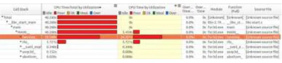
HOTSPOT ANALYSIS OF FOR3D

Using VTune Amplifier to analyze FOR3D and locate the hotspots. As shown in Figure 3, the hotspot of FOR3D is the subroutine twostep.

MULTI-THREADED PARALLEL TECHNOLOGY

This paper mainly uses OpenMP scheme which is a shared storage to accomplish the parallel computing[8]. In the outermost loops of FOR3D, there exists data dependency between different azimuth and depths. But there is no dependency between azimuth and the depth in the same range mentioned in line 7 in Figure. 2 which can be accomplished by adopting task parallelism[9]. In addition, the loops in the computing subroutines mentioned in line 8 in Figure 2 can be implemented by adopting data parallelism[10]. The parallel implementation of FOR3D is shown in Figure 4. The parts in the red dashed box are the main tasks for the OpenMP implementation.

Figure 4. The multi-thread parallel strategy of FOR3D.

MULTI-PROCESS OPTIMIZATION AND PARALLELIZATION OF FOR3D

The original FOR3D can only calculate the propagation loss of a single-frequency acoustic source underwater in a single run[11]. In this paper, we proposed a parallel implementation for calculating the propagation loss simultaneously when the acoustic source rays multiple-frequency by using MPI based on distributed storage. The parallel implementation steps are shown in Fig. 1. If we use the previous section of the OpenMP parallel computing for calculation of acoustic field in a specific frequency, we can achieve a hybrid MPI + OpenMP parallelization.

EXPERIMENTS AND ANALYSIS

Experiments Platform and Computer Environment

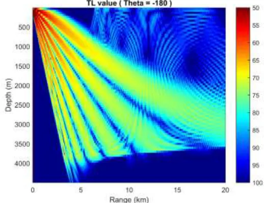
transmission loss in the case when 𝜃= -180° is shown in Figure 5. The computer environment for the experiments is shown in Table I.

Figure 5. Transmission loss calculation in horizontally stratified mediumusing FOR3D.

Results of Experiments

SERIAL OPTIMIZATION

A comparison of the results of the open source GNU Fortran compiler (gfortran) using the default option (-O0), with the commercial-grade Intel Fortran compiler (ifort) using the default option (-O2), is displayed in the first two rows in Table II. After changing the compiler, the performance of using the ifort compiler was improved more than 2 times. In the subsequent tests, we always use the ifort compiler. The result of selection of compiler options is also shown in Table II. Obviously, using -O3 -xHost –ipo is better than the other options.

A comparison of the elapsed time of part code, which solves the tri-diagonal matrix is shown in the first row in Table III. We found that the running time is reduced after our optimization. Using the performance-tuned math library MKL is 674s faster than the original code (about 11min).

The second row in TABLE III shows the elapsed time when running the entire program by using automatic vectorization and manual vectorization, respectively. In detail, the option -O2 is used when compiling the code optimized by manual vectorization. It can be seen that the effects of both vectorization schemes are very similar.

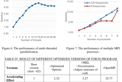
MULTI-THREADED PARALLELIZATION ON A SINGLE NODE

addition, too many threads’ forking and joining operations also increase the time cost. The parallel efficiency reaches the maximum in four-threads running. On the other hand, using 16 threads can reach the maximum speedup. The reason why the parallel efficiency is not high may be explained by the fact that the problem size as well as the total amount of calculations of the simulation is not so large, and the system overhead and proportion of non-parallel region of code are both increasing when more threads are employed.

TABLE I. CONFIGURATION OF EXPERIMENTAL HPC ENVIRONMENT.

Name Tianhe-2 Supercomputer

Node

Configuration

4 nodes×2CPU/node× 12cores/CPU× 2 hyper threads /core

CPU Intel(R) Xeon(R) E5-2692

v2:2.20G Hz

Operating

System Kylin Linux

Compiler GNU: gfortran(ver 4.4.7)

Intel: ifort(ver 14.0.2)

TABLE II. RESULT OF DIFFERENT COMPILING OPTIONS.

Options Time(s)

-O0(gfortran) 20400

-O0(ifort) 17160

-O2 8602

-O3 4643

-xHost 4415

-ipo 4577

-funroll-all-loops 5117

-parallel 7966

-O3 -ipo -xHOST 3705

TABLE III. TIME OF DIFFERENT OPTIMIZATION TESTS.

Optimization Methods Time(s)

Using math library for tri-diagonal system

NoMKL 2648

MKL 1974

Vectorization for range-stepping

No Vectorization 8602 Automatic

Vectorization 4477 Manual

Vectorization 4305

Figure 6. The performance of multi-threaded parallelization.

Figure 7. The performance of multiple MPI processes.

TABLE IV. RESULT OF DIFFERENT OPTIMIZED VERSIONS OF FOR3D PROGRAM.

Versions Base version (ifort –O2) +Optimized Options +MKL +Vectorization +Adjust structure of

code

+OpenMP

Accelerating

Effect 1 2.32 5.27 25.77

MULTI-PROCESS HYBRID PARALLELIZATION

To evaluate the performance gain of parallelization method introduced in section 3.2.3, several numerical experiments are conducted on the HPC machine. The problem size of the test case, expressed in the number of grid points, is 2000 (distance)  900 (azimuth)  6000 (depth), and the wide band signals composed of both 8 frequencies and 120 frequencies are tested.

At first, we only use MPI multi-process parallelization and each process is mapped into a physical CPU core in the simulation. The performance result is shown in Figure 7. We can observe that the running time of the program decreases rapidly as the number of processes increase, and a good speedup can be obtained, especially in the 120-frequency case. However, in the 8-frequency case, there are only eight tasks to be assigned to multiple processes of which the number is varying from 1 to 8. This results in a low speedup due to severe lack of balance of the workloads among these processes. It is worthy to note that a super-linear speedup can be obtained in the case of 120 frequencies, which is due to the fact that multiple-process can make full use of the memory system of the single node. More data can be loaded into the memory all at once when using multiple processes, thus better data locality of the data access can be achieved.

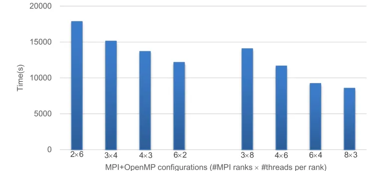
In the following test, the OpenMP multi-threaded and multi-process hybrid parallelization method are used, and the performance result is reported in Figure 8. The number of frequencies is 120, in these numerical simulation cases. It shows that different configurations of processes and threads have different performance results even if the number of total processor cores remains the same. We can also compare the accelerating effects of the multi-process technique and the multi-threaded approaches. For example, when taking the “3 MPI ranks (processes)  4 threads per rank” configuration (“3  4” shown in Fig. 8) as the baseline, doubling the number

0.00 1.00 2.00 3.00 4.00 5.00

1 2 3 4 6 8 10 12 16 20 24 32 36 48

S

pe

ed

up

Number of threads

0.00 5.00 10.00 15.00

1 2 3 4 5 6 7 8

S

pe

ed

up

of MPI processes, i.e. “6  4” configuration, results in a parallel efficiency of 1.64, whereas doubling the number of threads per rank, i.e. “3  8” configuration, results in a parallel efficiency of 1.08. It’s obvious that doubling the number of MPI processes gives a better performance than doubling the number of threads. The same conclusion can be drawn from other configurations. The main reason is that the multi-process implementation is a coarse-grain parallelization, which aims to partition the loads of different frequencies. By contrast, the multi-threaded implementation has fine-grain parallelism, which aims to accelerate the nested loops.

Figure 8. Performance of MPI+OpenMP hybrid parallelization for simulating the propagation of wide band underwater signals.

CONCLUSIONS

Using high-performance computers is an effective way to improve the efficiency for calculations of the acoustic field. In this paper, we propose a series of parallelization and optimization methods to improve the performance of the three-dimensional parabolic equation solver and achieve good results. Based on the optimization results of single node, the multi-frequency parabolic equation solver implemented using OpenMP+MPI hybrid parallelization. The proposed parallelization and optimization methods can be easily extended to the distributed-memory environment composed of multiple nodes, and our work is helpful to the large-scale acoustic applications with real-time requirement.

ACKNOWLEDGEMENT

This work is supported by National Key R&D Program of China (2016YC1401800), National Natural Science Foundation of China (61379056), and Natural Science Foundation of Hunan Province, China (2017JJ2305).

26 34 43 62 38 46 64 83

0 5000 10000 15000 20000

Tim

e(

s)

REFERENCES

1. Finn B. Jensen, William A. Kuperman, Michael B. Porter and Henrik Schmidt. 2011.

Computational Ocean Acoustics Second Edition. Springer, New York Dordrecht Heidelberg London, pp.15-27.

2. J.B.Keller. 1978. “Rays, waves and asymptotics,” Ball.Am.Math.Soc.84:727-750.

3. D. Lee and W.L. Siegmann. 1986. “A Mathematical Model for the 3-Dimensional Ocean Sound Propagation,” Mathematical Modelling, 7:143-162.

4. D. Lee, G. Botseas and J.S. Papadakis. 1981. “Finite-Difference Solutions to the Parabolic Wave Equation,” Journal of the Acoustical Society of America, 70(3):795-800.

5. R.N. Baer. 1981. “Propagation through a Three-Dimensional Eddy Including Effects on an Array,” Journal of the Acoustical Society of America, 69:70-75.

6. Ding L., Botseas G. and Siegmann W. L. 1992. “Examination of three dimensional effects using a propagation model with azimuth́ coupling capability (FOR3D),” The Journal of the Acoustical Society of America, 91(6): 3192-3202.

7. Botseas G., Lee D. and King D. 1987. “FOR3D: A Computer Model for Solving the LSS Three-Dimensional, Wide Angle Wave Equation,” NUSC Technical Report 7943, Naval Underwater Systems Center, New London, CT.

8. Chen Guoliang, An Hong, Chen Ling, Zheng Qilong and Shan Jiulong. 2004. “Practice of Parallel Algorithms,” Higher Education Press, pp.158-181.

9. Castor K. and Sturm F. 2008. “Investigation of 3D acoustical effects using a multiprocessing parabolic equation based algorithm,” Journal of Computational Acoustics, 16(2):137-162. 10. Wang Lujun and Peng Zhaohui. 2009. “Parallel computation of sound field by OpenMP-based

PE model,” Technical Acoustics, 28(3): 227-232.