An Evidential Reasoning-based Decision Support
System to Support House Hunting
Tanjim Mahmud
Dept.of Computer Science & Engineering University of Chittagong Chittagong, Bangladesh
Mohammad Shahadat Hossain
Dept.of Computer Science & Engineering University of Chittagong Chittagong, Bangladesh
ABSTRACT
House hunting meaning the activity of trying to find a house to live in, is considered as one of the most important activities for many families worldwide. This involves many criterions/factors to be measured and evaluated. These factors are expressed both in quantitative and qualitative ways. In addition, a hierarchical relationship exists among the factors. Moreover, it is difficult to measure qualitative factors in an objective/quantitative way, resulting incompleteness in data and hence, uncertainty. Therefore, it is necessary to address the issue of uncertainty by using appropriate methodology; otherwise, the decision to select a house to live in will become inappropriate. There exist many methods such as Analytical Hierarchical Process (AHP), Analytical Network Process (ANP), Inner Product Vector (IPV) to address the issue presented in this paper. However, none of them is able to address the issue of uncertainty and hence, resulting inappropriate selection of a house to live in. Therefore, this paper demonstrates the application of a novel method named Evidential Reasoning (ER), which is capable of addressing the uncertainty of multi-criterion problem, where there exist factors of both subjective and quantitative nature. The ER approach handles uncertainties by using a belief structure, the evidential reasoning approach used in aggregating degrees of belief from lower level attributes to higher level attributes [7]. This paper reports the development of DSS using ER approach, which is capable of providing overall assessment on the location of a house to live in taking account of both qualitative and quantitative factors. Chittagong, which is the second largest city of Bangladesh has been considered as the case study area to demonstrate the application of the developed DSS..
Keywords
Multiple criteria decision analysis (MCDA), uncertainty, evidential reasoning (ER), Analytical hierarchy process (AHP), Decision support system (DSS)
1.
INTRODUCTION
House hunting involves multiple criterions (such as, location, safety, attractiveness, environment, proximity to different services, property insurance, utility cost, maintenance cost, house cost per square feet), which are quantitative and qualitative in nature. Numerical data which uses numbers is considered as quantitative data and can be measured with 100% certainty.[4] Examples of quantitative data property insurance, utility cost, maintenance cost, house cost per square feet are the examples of quantitative data since they can be measured using number and with 100% certainty. On the other hand, qualitative data is descriptive in nature, which defines some concepts or ill-defined characteristics or quality of things [5].Hence, this data can’t describe a thing with
addressed and more accurate and robust decision can be made. The ER approach has addressed such issue by proposing a belief structure which assign degree of belief in the various evaluation grades of the attributes, which is not the case in AHP in other multi-criterions decision techniques. For example ANP,IPV[20]
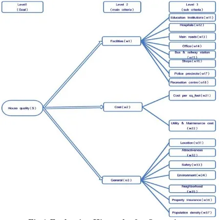
Fig 1:Evaluation Hierarchy for Operation.
In section 2 will briefly represent ER algorithm. Section 3 will demonstrate the application of ER in house hunting problem. Section 4 will represent the results and achievement. Finally section 5 will conclude the research.
2.
EVIDENTIAL REASONING
APPROACH
The evidential reasoning algorithm is considered as the kernel of the ER approach. This algorithm has been developed based on an evaluation analysis model [22][23] and the evidence combination rule of the Dempster-Shafer (D-S) theory [15][18][19], which is well-suited for handling incomplete uncertainty [22]. The ER approach uses a belief structure to model an assessment as a distribution. It differs with other Multi Criteria Decision Making (MCDM) modeling methods in that it employs evidence-based reasoning process to derive a conclusion [13][14][20]. The main strength of this approach is that it can handle uncertainties associated with quantitative and qualitative data, related to MCDM problems[13][14] [20]. The ER approach consists of five phases including 1) Information acquisition and representation or assessment, 2) weight normalization, 3) basic probability assignment 4) attribute aggregation, 5) Combined degree of belief calculation, 6) utility function 7) ranking
2.1
Assessment
One of the critical tasks of developing a decision support system is to acquire information and to represent them in appropriate format so that it will feed into a model. Since ER approach employs belief structure to acquire knowledge, appropriate information should be selected to feed the ER algorithm, which is used to process the information.
Let ‘house quality’ (S) be an attribute at level 1 as shown in Fig. 1, which is to be assessed for an alternative (A) (i.e. a house at a certain location) and this assessment can be
denoted by A(S). This is to be evaluated based on a set of wi sub-attributes (such as facilities, cost, general) at level 2,
denoted by:
S
{
w
1,
w
2,
w
3,...
..
w
i,...
w
n}
. House quality (S) can be assessed by using a set of evaluationgrades consisting of
)
(
),
(
)
(
),
(
H
1Good
H
2Average
H
3Bad
H
4Excellent
and this set can be written as
}
,...,
2
,
1
,
,...
,
{
H
1H
2H
n
N
H
n
. Theseevaluation grades are mutually exclusive and collectively exhaustive and hence, they form a frame of discernment in D-S terminology.
A degree of belief is associated with each evaluation grade,
which is denoted by
{(
H
n,
n),
n
1
,...,
N
}
Hence,}
,...,
1
),
,
{(
)
(
S
H
n
N
A
n
n
denotes that the topattribute S is assessed to grade
H
n with the degree of beliefn
. In this assessment, it is required that
n
0
and1
1
N
n n
. If1
1
N
n n
the assessment is said to becomplete and if it is less than one then the assessment is
considered as incomplete. If
0
1
N
n n
then theassessment stands for complete ignorance. In the same way,
sub-attribute
w
i is assessed to gradeH
n with the degree of belief
n,iand this assessment can be represented as
}
,...,
1
,...,
1
),
,
{(
)
(
w
H
,n
N
and
i
n
A
i
n
ni
Such that
n,i
0
and1
1
N
n n
.The incompleteness as mentioned occurs due to ignorance, meaning that belief degree has not been assigned to any specific evaluation grade and this can be represented using the equation as given below.
Nn n H
1
1
……….. (1)
Where
H is the belief degree unassigned to any specificgrade. If the value of
H is zero then it can argued that thereis an absence of ignorance or incompleteness. If the value of
H
is greater than zero then it can be inferred that there [image:2.595.56.280.139.364.2]However, when a hospital is located 1.3 km of the house, it can be both excellent and average. However, it is important for us to know, with what degree of belief it is excellent and with what degree of belief it is average. This phenomenon can be calculated with the following formula.
i n i
n i n n
n i n
h
i
h
h
h
, ,
1 , 1
1
,
,
1
,
)
2
...(
, 1 ,i n i
n
h
h
h
if
Here, the degree of belief
n,i is associated with theevaluation grade ‘average’ while
n1,i is associated with the upper level evaluation grade i.e. excellent. The value of hn+1 is the value related to excellent, which is considered as1km i.e. the location of the hospital. The value of
h
n1 is related to average, which is 1.5 km. Hence, applying equation (2) the distribution of the degree of belief with respect to 1.3 Km of the location of the hospital from the house can be assessed by using equation (2) and the result is given below:{(Excellent, 0.4), (Good, 0.6), (Average, 0), (Bad,0)}
2.2
Weight Normalization
The identification of the importance of the attributes is very important, since each attribute does not play the same role in decision making process. For example, the sub-attribute of the “Facilities” attribute at level 2 consists of eight attributes namely, proximity to educations institutions, main road, hospitals, shops, office, bus and railway station, police precincts, recreation centre. It is important for us to know among eight attributes which is the most important in evaluating their parent attribute “Facilities”. This can be carried out by employing different weight normalization techniques such as Eigenvector, AHP, Pair wise comparison [8][9][16][17]. In this research Pair wise comparison method has been considered for the normalization of the weights of the attribute by considering the following equations
..
ji i i i
y
y
1
;i= 1…….j……(3)
Li i 1
1
……(4)Equation (3) is used to calculate the importance of an attribute
)
(
w
i.. This has been calculated by dividing the importance
of an attribute
(
y
i)
(this important of the attribute has beendetermined from survey data) by the summation
j
i i
y
1of
importance of all the attributes. Equation (4) has been used to check whether the summation of the importance of all the attributes is within one i.e whether they are normalized.
2.3
Basic probability assignment
The degrees of belief as assigned to the evaluation grades of the attributes need to be transformed into basic probability masses. Basic probability mass measures the belief exactly assigned to the n-th evaluation grade of an attribute. It also represents how strongly the evidence supports n-th evaluation
grade
(
H
n)
of the attribute. The transformation can beachieved by combining relative weight
(
w
i)
of the attributewith the degree of belief
(
n,i)
associated with n-thevaluation grade of the attribute, which is shown by the
following equation.
m
n,i
m
i(
H
n)
w
i
n,i(
a
l),
‘’’’;
,...,
1
N
n
’’’’’’’’’’
,
....,
,...
1
L
i
……….(5)
However, in case of hierarchical model, the basic probability mass represents the degree to which the i-th basic attribute supports the hypothesis that the top attribute y is assessed to n-th evaluation grade.
The remaining probability mass unassigned to any individual grade after the ith attribute has been assessed can be given using the following equation.
Nn
l i n N
n i n i
i
H
m
H
m
w
a
m
1 , 1
,
,
(
)
1
1
(
),
,
....,
,...
1
L
i
…….(6)2.4
ER algorithm (Kernel of ER approach)
The purpose of ER algorithm is to obtain the combined degree of belief at the top level attribute of a hierarchy based on its bottom level attributes, also known as basic attributes. This is achieved through an effective process of synthesizing/aggregating of the information. A recursive ER algorithm is used to aggregate basic attributes to obtain the combined degree of belief of the top level attribute of a hierarchy, which can be represented as
}
,...,
1
),
,
{(
)
(
S
H
n
N
A
n
n
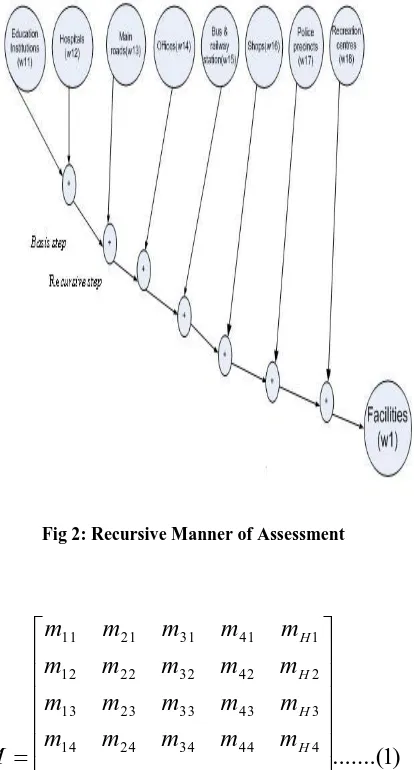
. In this recursiveER algorithm, all the basic attributes are aggregated recursively in the following manner as shown in Fig. 2.
In this Fig.2 “Facilities” is considered as the top level attribute, which consists of eight sub-attributes. The top level attribute “Facilities” can be denoted by w(i) such that i= 1,2,3,..n. This means at this level there could be other attributes. For example, in our case, this level consists of three attributes and the level is considered as second level as shown in Fig. 1. It is interesting to note that top level of Fig.1 contains only one attribute and that can be denoted by So (House Quality) and has three sub-attributes at second level. For the top level attribute (S) the combined degree of belief needs to be calculated based on the second level attributes. From Fig.2 it can be observed that w(1), [considering the value of i as 1] consists of eight sub- attributes and hence
}
...
,...
,
,
{
11 12 13 181
w
w
w
w
w
or
i
{
w
i,j,
w
i,j 1,
w
i,J 2,...
...
w
i,J n}
w
such thati=1…..n and j = 1…..L. Taking account of the basic probability assignment and remaining unassigned probability
mass of eight sub-attributes mass of
w
1 matrix (1) has beendeveloped as shown below. These bpa (such as m11, m21,,etc and reaming unassigned bpa such MH1) have been calculated by using equations 5 and 6.
.
Fig 2: Recursive Manner of Assessment
From matrix (1), it can be seen that each sub-attribute is
associated with five basic probability assignment(bpa), where
four first four bpa
(
m
11,
m
21,
m
31,
m
41)
are associated with four evaluation grades(
H
1,
H
2,
H
3,
H
4)
and finalbpa i.e.
m
H,i is showing the remaining probability mass unassigned to any individual grades after the assessments on sub-attribute have been considered. Each row in this matrix represents bpa related to one basic attribute or sub-attribute.Now it is necessary to aggregate the bpa of different sub-attributes. The aggregation is carried out in a recursive way. For example, the bpa of first sub-attribute attribute (which is shown in the first row of the matrix 1) is aggregated with the bpa of second sub-attribute. The result of this aggregation is illustrated in the first row of the matrix (2) and this can be considered as the base case of this recursive procedure since this will be used in the latter aggregation of the sub-attributes. This aggregation can be achieved by using the following equation, which will yield combined bpa (such as
) 2 ( 4 ) 2 (
1I
,...
...
m
Im
) as shown in the first row of thesecond matrix.
)
(
11 12 1 12 2 11 ) 2 ( ) 2 (1
K
m
m
m
m
m
m
m
I
I
H
H…………(7)
Similarly
m
2I(2),
m
3I(2),
m
4I(2)can be calculated.Where
K
I(2) is a normalization factor used to resolve the conflict and this can be calculated using the equation (8). [image:4.595.69.271.584.704.2])
8
...(
...
1
,...,
1
,
1
1 1 1 1 , ) ( , ) 1 (
m
m
i
L
K
N n N n t t i t i I n i IThe aggregation of the third attribute is carried out with the resultant of the aggregation of the bpa of the first two attributes. In this way, the aggregation of the other attributes is carried out and finally, the combined aggregations of all the attributes are obtained. This phenomenon has been depicted in Figure 2, where the combined aggregation is obtained, which will be used to obtain the combined degree of belief for the second level attribute “facilities”. Equation (9) represents the more generalized version of equation (7)
,() , 1 ,() , 1 ,() , 1
) 1 ( ) 1 ( ,
:
Ii nIi ni
nIi Hi
HIi nii I n n
m
m
m
m
m
m
K
m
H
………….(9) ), ( , ) ( , ) (,Ii HIi
~
HIiH
m
m
m
n
1
,...
....,
N
,
………..(10)
,() , 1 ,() , 1 ,() , 1
) 1 ( ) 1 ( ,
~
~
~
~
~
:
Ii HIi Hi
HIi Hi
HIi Hii I
H
K
m
m
m
m
m
m
m
H
…….(11)
H
:
m
H,I(i1)
K
I(i1)
m
H,I(i)m
H,i1
,
…….. (12)
Equation 13 is used to calculate the combined degree of belief
by using final combined basic probability assignment, say in
this case “facilities”.
,
1
,...
,.
,
1
:
) ( ,
) ( ,
N
n
m
m
H
L I H
L I n n
n
….(13)
,
1
~
:
) ( ,
) ( ,
L I H
L I H H
m
m
H
Where)
,...
1
(
1 , ) 1 (
,
m
n
N
m
nI
n
……..….(14)
n
and
H represent the belief degrees of the aggregatedassessment, to which the general factor (such as “facilities”)
is assessed to the grade
H
n and H, respectively. Thecombined assessment can be denoted by
(
)
,
1
,...,
.
))
(
(
y
a
H
,a
n
N
S
l
n
n l
, . It has
been proved that
1
H
1
Nn
n
The recursive ER algorithm combines various piece of evidence on a one-by-one basis.
2.5
The Utility Function (Ranking house)
Utility function is used to determine the ranking of the different alternatives. In this research houses at five locations have been considered as the alternatives. Therefore, the determination of ranking of the alternatives will help to take a decision to decide the suitable location of a house. There are three different types of utility functions considered in the ER approach namely: minimum utility, maximum utility and average utility. In this function, a number is assigned to an evaluation or assessment grade. The number is assigned by taking account of the preference of the decision maker to a certain evaluation grade. Suppose the utility of an evaluation
grade
H
n isu
(
H
n)
, then the expected utility of the aggregated assessmentS
(
y
(
a
l))
is defined as follows:
Nn
l n n
l
u
H
a
a
y
S
u
1
)
(
)
(
)))
(
(
(
The belief degree
n(
a
l)
represents the lower bound ofthe likelihood that
a
lis assessed toH
n, whilst the corresponding upper bound of the likelihood is given by))
(
)
(
(
na
l
Ha
l The maximum, minimum and average utilities ofa
l can be calculated by:)),
(
))
(
)
(
(
)
(
)
(
)
(
1
1
max n N l H l N
N
n l n
l
a
u
H
a
a
u
H
a
u
),
(
)
(
)
(
))
(
)
(
(
)
(
2 1 1
min n
N
n l n l
H l
l
a
a
u
H
a
u
H
a
u
.
2
)
(
)
(
)
(
max l min ll average
a
u
a
u
a
u
It is important that if
u
(
H
1)
0
, then)
(
)))
(
(
(
S
y
a
lu
mina
lu
if all the original assessments))
(
(
e
ia
lS
in the belief matrix are complete, then0
)
(
l
Ha
and).
(
)
(
)
(
)))
(
(
(
S
y
a
lu
mina
lu
mina
lu
averagea
lu
It has to be made clear that the above utilities are only used for characterizing a distributed assessment but not for the aggregation of factors.
3.
RESULTS AND DISCUSSION
In the previous section, we have discussed about the ER method and how to implement it. Therefore, in this section we will look at the results from using this method on the house quality in Chittagong[24] is a beautiful city with its city center facing the port. Many families migrate to Chittagong due to the fact that it provides a nice and safe environment. It is however, difficult to find the perfect area to live in without thorough research of the neighborhoods in the city. The ER approach for house hunting consists mainly of four key parts, which are the identification of factors, the ER distributed modeling framework for the identified factors, the recursive ER algorithms for aggregating multiple identified factors, and the utility function [3] based ER ranking method which is designed to compare and rank alternatives/options systematically. Each part will be described in detail in this section. House quality, can be described in two broad categories: the Objective attribute, and subjective attribute as shown in Fig. 1 and each attribute weights are
[image:5.595.54.274.144.359.2]w11=0.09,w12=0.03,w13=0.01,w14=0.02,w15=0.02,w16=0.0 1,w17=0.02,w18=0.01,w21=0.01,w22=0.02,w31=0.12,w32=0 .14,w33=0.30,w34=0.15,w35=0.02,w36=0.01,w37=0.11
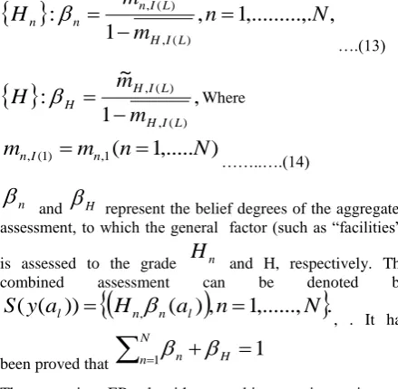
Table 1 shows the assessment grades defined by the decision maker for Level 3(Figure 1:).Table 2 shows the assessment distribution which must be done first by employing the transformation equation. Any measurements of quality can be translated to the same set of grades as the top attribute which make it easy for further analysis. The assessments given by the Decision Maker (DM) in Figure 1: are fed into Decision support system (DSS)[25][26] and the aggregated results are yielded at the5main criteria level (Figure 1:). The assessment grades for each main criterion are abbreviated in Table 1 . The numbers in brackets show the degrees of belief of the DM that are aggregated from the assessments of the sub-criteria. One can rank the house for each criterion in order of preference by comparing the distributed assessments shown in Table 2.
Table 1
Assessment grades defined by the decision maker for the 3rd level
Excellent Good Average Bad Excellent Good Average Bad Excellent Good Average Bad Excellent Good Average Bad Excellent Good Average Bad
Quantitative Quantitative Quantitative Quantitative Quantitative Quantitative Quantitative Assessment grades
Quantitative Quantitative Quantitative Quantitative Quantitative
Proximity to Main Road Police Precincts Property Insurance Population Density Cost per Square Feet Utility & Maintanence Cost Proximity to Education Institutions
Proximity to Hospitals Proximity to Shops Proximity to Office Proximity to Bus & Railway Station
Proximity to Recreation Centre Nice Neighborhood
Attributes Location Attactiveness
Safety Environment
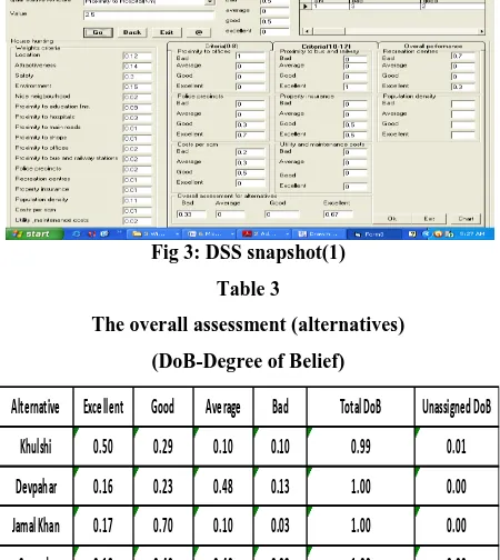
For instance, the results for House Khulsi can be interpreted as follows: House Khulsi is assessed to be 15% bad, 10% average, 23% good, and 52% excellent. The total degree of belief does not add up to one (or 100%) as a result of incomplete and/or missing assessments. The results in Table 2 are supported by a graphical display (Figure 3:). The house could be ranked in order of preference by comparing them with each other as in Table 1. However, a comparison may not be possible when house have very similar degrees of belief assigned to each grade, such as house Khulsi and Jamal khan (see Table 3). One way to solve this problem is to quantify the grades. There are several ways of quantifying grades. One of them is to assign a utility for each grade and
then obtain an expected utility for each house. Then, house are ranked based on their expected utility[3]. In this research, the former approach is used. A number of hypothetical lottery type questions were presented to the DM in order to establish preference among grades. The following utilities are assigned to each grade:
(Bad, 0.4),( Average , 0.7), (Good ,0.85) and (Excellent , 1)
The total Degree of belief for each House in Table 3 does not add up to one, because some of the assessments were incomplete and missing. For example, the total Degree of belief assigned to house alternative is 97%. That is, there is a 3% unassigned degree of belief. The DSS uses the concept of utility interval to characterize the unassigned Degree of belief (or ignorance) which can actually fall into any grade. The ER algorithm generates a utility interval enclosed by two extreme cases where the unassigned Degree of belief goes either to the least preferred grade (minimum utility) or goes to the most preferred grade (maximum utility). The minimum and maximum possible utilities of each alternative generated by the DSS[25][26] (based on the given utility values for each grade above) are shown in Table 4 or Figure 5:. For example, the results for house Khulsi from TABLE 3 are as follows: House Khulsi is minimum utility .
{[(Degree of belief assigned under grade bad + unassigned Degree of belief) utility of grade bad] + (Degree of belief assigned under grade average * utility of grade average) + (Degree of belief assigned under grade good *utility of grade good) + (Degree of belief assigned under grade excellent * utility of grade excellent)}.
Hence, House Khulsi minimum utility .
{[(0.1+ 0.01) 0.4] + (0.1 * 0.7) + (0.29 *0.85)+ (0.5 *1.0 ) =0.860
House Khulsi's maximum utility . {(Degree of belief assigned under grade bad* utility of grade bad) + (Degree of belief assigned under grade average* utility of grade average) + (Degree of belief assigned under grade good* utility of grade good) + [(Degree of belief assigned under grade excellent + unassigned Degree of belief) *utility of grade excellent]}.
Table 2
Assessment scores of houses based on sub criteria (E-Excellent,G-Good,A-Average,B-Bad)
Khulshi Devpahar Jamal khan Suganda Chandgoan
B(0.2)A(0.8) G(0.4)E(0.6) G(0.4)E(0.6) E(1.0) G(0.4)E(0.6)
G(0.4)E(0.6) B(0.2)A(0.8) B(0.2)A(0.8) G(0.4)E(0.6) E(1.0)
B(0.2)E(0.8) A(1.0) G(1.0) A(1.0) B(0.2)A(0.8)
E(1.0) G(1.0) G(0.4)E(0.6) G(1.0) G(0.4)E(0.6)
G(1.0) B(0.2)E(0.8) E(1.0) B(0.2)A(0.8) G(1.0)
2.1 3.0 2.0 1.9 1.7
2.3 2.6 2.4 2.0 3.0
1.5 2.0 1.0 2.9 1.6
2.0 1.6 1.0 2.0 3.0
3.0 2.0 2.1 2.5 2.7
1.0 2.0 2.6 1.7 1.9
1.4 1.0 2.1 2.5 2.8
1.8 1.4 1.4 1.8 1.3
1.0 1.6 1.6 2.0 3.0
2.0 1.0 2.0 1.0 3.0
2.3 1.0 1.1 1.4 1.3
Nice Neighborhood Attributes
Location Attactiveness
Safety Environment
Cost per Square Feet(Thousand) Proximity to Education Institutions(Km)
Proximity to Hospitals(Km) Proximity to Shops(Km) Proximity to Office(Km) Proximity to Bus & Railway Station(Km)
Proximity to Recreation Centre(Km) Proximity to Main Road(Km)
Police Precincts(Km) Property Insurance(Crore)
[image:6.595.62.537.560.730.2]Fig 3: DSS snapshot(1) Table 3
The overall assessment (alternatives) (DoB-Degree of Belief)
Alternative Excellent Good Average Bad Total DoB Unassigned DoB Khulshi 0.50 0.29 0.10 0.10 0.99 0.01 Devpahar 0.16 0.23 0.48 0.13 1.00 0.00 Jamal Khan 0.17 0.70 0.10 0.03 1.00 0.00 Suganda 0.18 0.40 0.40 0.02 1.00 0.00 Chandgoan 0.28 0.17 0.33 0.22 1.00 0.00
Hence, House Khulsi maximum utility
{(0.1* 0.4)+ (0.1 * 0.7) + (0.29 *0.85)+[ (0.5 +0.01)*1.0 ]} =0.866
Fig 4: DSS snapshot (2). Table 4
The expected utilities of alternative house
Alternative Minimum Utility
Maximum Utility
Average Utility
Rank
Khulsi 0.860 0.866 0.863 1
Dev Pahar 0.743 0.743 0.743 4or 5
Jamal khan 0.847 0.847 0.847 2
Suganda 0.808 0.808 0.808 3
Chandgoan 0.743 0.743 0.743 5or 4
House Khulsi’s average utility . (maximum utility + minimum utility)/2 =0.863
Fig 5: Expected average utility of alternative.
The house may be ranked based on the average utility but this may be misleading. In order to say that one house theoretically dominates another, the preferred house's minimum utility must be equal or greater than the dominated house's maximum utility. For example, based on an average utility, house Jamal khan is preferred to house Khulsi. The DM's request for simplicity, average utilities are used to rank houses. The ranking of houses is as follows:
Khulsi > Jamal khan > Suganda >Dev Pahar >Chandgoan or Khulsi > Jamal khan > Suganda > Chandgoan >Dev Pahar
4.
CONCLUSION
This paper introduced an application of evidential reasoning to solve a multiple criteria house hunting problems with uncertain, incomplete, imprecise, and/or missing information. From the results shown above, it is reasonable to say that the ER method is a mathematically sound approach towards measuring the house quality as it employs a belief structure to represent an assessment as a distribution. This approach is quite different from the other Multi Criteria Decision Making model such as the Saaty ’s AHP method which uses a pair wise comparison matrix[8][9][13[14]. Hence, the ER can handle new attribute without recalculating the previous assessment because the attribute can be arranged or numbered randomly which means that the final results do not depend on the order in which the basic attributes are aggregated. Furthermore, any number of new houses can be added to the assessment as it does not cause a ‘rank reversal problem’ as in the Saaty’s AHP method[8][9][13[14]. Finally, in a complex assessment as in the house quality assessment which involved objective and subjective assessments of many basic attributes as shown in Figure 1, it is convenient to have an approach which can tackle the uncertainties or incompleteness in the data gathered. Therefore, the ER is seen as feasible method for quality assessment.
5.
REFERENCES
[1] M Sonmez, G. Graham and J. B. Yang and G D Holt, “Applying evidential reasoning to pre-qualifying construction contractors”, Journal of Management in Engineering, Vol.18, No.3, pp.111-119, 2002.
[2] J. B. Yang, “Rule and utility based evidential reasoning approach for multiple attribute decision analysis under
0.65 0.7 0.75 0.8 0.85 0.9
A
ve
rag
e
u
til
ity
[image:7.595.56.283.422.606.2] [image:7.595.55.280.626.713.2]uncertainty”, European Journal of Operational Research, Vol. 131, No.1, pp.31-61, 2001.
[3] Y. M. Wang, J. B. Yang and D. L. Xu, “Environmental Impact Assessment Using the Evidential Reasoning Approach”, European Journal of Operational Research, Vol.174, No.3, pp.1885-1913, 2006.
[4] Lisa M. (2008). The Sage encyclopedia of qualitative research methods. Los Angeles, Calif.: Sage Publications. ISBN 1-4129-4163-6.
[5] http://www.pearson.ch/1449/9780273722595/An-Introduction-to-Geographical.aspx
[6] Dodge Y. (2003) The Oxford Dictionary of Statistical Terms, OUP. ISBN 0-19-920613-9
[7] D. L. Xu and J. B. Yang, “Introduction to multi-criteria decision making and the evidential reasoning approach”, Working Paper Series,Paper No.: 0106 , ISBN: 1 86115 111 X (http://www.umist.ac.uk/management), Manchester School of Management, UMIST, pp. 1-21, 2001.
[8] Saaty, T.L. (1980). The Analytic Hierarchy Process: Planning, Priority Setting, Resource Allocation. New York: McGraw-Hill,.
[9] Grandzol, John R. (August 2005). "Improving the Faculty Selection Process in Higher Education: A Case for the Analytic Hierarchy Process" . IR Applications 6. Retrieved 2007-08-21.
[10] Atthirawong, Walailak; Bart McCarthy (September, 2002). "An Application of the Analytical Hierarchy Process to International Location Decision-Making". In Gregory, Mike. Proceedings of The 7th Annual Cambridge International Manufacturing Symposium: Restructuring Global Manufacturing. Cambridge, England: University of Cambridge. pp. 1–18.
[11] Larson, Charles D.; Ernest H. Forman (January, 2007). "Application of the Analytic Hierarchy Process to Select Project Scope for Videologging and Pavement Condition Data Collection". 86th Annual Meeting Compendium of Papers CD-ROM. Transportation Research Board of the National Academies.
[12] Drake, P.R. (1998). "Using the Analytic Hierarchy Process in Engineering Education" . International Journal of Engineering Education 14 (3): 191–196. Retrieved 2007-08-20.
[13] Köksalan, M., Wallenius, J., and Zionts, S. (2011). Multiple Criteria Decision Making: From Early History to the 21st Century. Singapore: World Scientific.
[14] Köksalan, M.M. and Sagala, P.N.S., M. M.; Sagala, P. N. S. (1995). "Interactive Approaches for Discrete Alternative Multiple Criteria Decision Making with Monotone Utility Functions". Management Science 41 (7): 1158–1171.
[15] A. Taroun and J. B. Yang. "Dempster-Shafer theory of evidence: potential usage for decision making and risk analysis in construction project management." Journal of the Built and Human Environment Review 4, no. 1(2011) : 155-166
[16] Saaty, Thomas L. (2008). Decision Making for Leaders: The Analytic Hierarchy Process for Decisions in a Complex World. Pittsburgh, Pennsylvania: RWS
Publications. ISBN 0-9620317-8-X.
http://www.amazon.com/dp/096203178X.
[17] Dey, Prasanta Kumar (November 2003). "Analytic Hierarchy Process Analyzes Risk of Operating Cross-Country Petroleum Pipelines in India". Natural Hazards Review 4 (4): 213–221. DOI:10.1061/(ASCE)1527-6988(2003)4:4(213)
[18] L. Zadeh, A simple view of the Dempster-Shafer Theory of Evidence and its implication for the rule of combination, The Al Magazine, Vol. 7, No. 2, pp. 85-90, Summer 1986.
[19] Kari Sentz and Scott Ferson (2002); Combination of Evidence in Dempster–Shafer Theory, Sandia National Laboratories SAND 2002-0835
[20] Saaty, Thomas L. (1996). Decision Making with Dependence and Feedback: The Analytic Network Process. Pittsburgh, Pennsylvania: RWS Publications. ISBN 0-9620317-9-8.
[21] Bragge, J.; Korhonen, P., Wallenius, H. and Wallenius, J. (2010). "Bibliometric Analysis of Multiple Criteria Decision Making/Multiattribute Utility Theory". IXX International MCDM Conference Proceedings, (Eds.) M. Ehrgott, B. Naujoks, T. Stewart, and J. Wallenius,. Springer, Berlin 634: 259–268.
[22] P. Sen and J. B. Yang, "Design decision making based upon multiple attribute evaluation and minimal preference information", Mathematical and Computer Modelling, Vol.20, No.3, pp.107-124, 1994.
.[23] B. Yang and P. Sen, "Multiple attribute design evaluation of large engineering products using the evidential reasoning approach", Journal of Engineering Design, Vol.8, No.3, pp.211-230, 1997
[24] List of cities and towns in Bangladesh, Retrieved December 29, 2009
[25] Henk G. Sol et al. (1987). Expert systems and artificial intelligence in decision support systems: proceedings of the Second Mini Euroconference, Lunteren, The Netherlands, 17–20 November 1985. Springer, 1987. ISBN 90-277-2437-7. p.1-2.