Solving Single Machine Total Weighted Tardiness
Problem using Variable Structure Learning Automata
Saeed Sabamoniri
Computer Engineering Departement, Islamic AzadUniversity, Sofian Branch, Sofian, East Azarbayjan, Iran
Kayvan Asghari
Computer Engineering Departement, Islamic Azad University, Khameneh Branch, Khameneh, East Azarbayjan, IranMohammad Javad Hosseini
Computer Engineering Departement, Islamic AzadUniversity, Sofian Branch, Sofian, East Azarbayjan, Iran
ABSTRACT
In this paper intelligent search technique of variable structure learning automata (VSLA) has been used to solve single machine total weighted tardiness job scheduling problem. The goal is investigating reduction in delays result in late execution of the jobs after specified deadline as well as reducing the time required to find the best execution order of the jobs. For this reason, fixed structure learning automata and genetic algorithm approaches has been studied and then a new scheduling approach called VSLA-Scheduler has been proposed by employing variable structure learning automata technique. In order to identify strengths and weaknesses of the proposed method, its performance is compared with other intelligent techniques. In this regard, for performance evaluation of the proposed method and comparing it with other methods, computer simulations have been used. Finally, the results produced by the proposed and previous algorithms have been compared with the best solutions in OR library. Experimental results show that the proposed algorithm's performance (VSLA-Scheduler) is more acceptable than other methods.
General Terms
Scheduling, single machine task scheduling, machine learning.
Keywords
Total Weighted Tardiness Scheduling, Learning Automata, Genetic Algorithms, Object Migration LA.
1.
INTRODUCTION
There are many problems which finding optimal solution for them with Polynomial time complexity algorithm is impossible and they require some algorithms with exponential time complexity. In these problems by increasing the input size of the problem, the time required to obtain the optimal solution, exponentially increases. The single machine total weighted tardiness (SMTWT) problem is one of these kinds of problems. In this paper, single-machine scheduling problem has been studied. The aim of this problem is minimizing total weighted tardiness of jobs which exist in an execution sequence. In this problem it must be executed n jobs on one machine sequentially. Each job i has a related processing time called Pi, a weight Wi, and a due date as di which are available for processing.
Tardiness of job i is defined as Ti= max {0, Ci-di} which Ci is completion time for job i in the current jobs sequence. In this problem the goal is to find a sequence of jobs such that the total weighted tardiness (
n
i 1
w
i.
T
i) minimized. For arbitrary positive weights, SMTWT problem is stronglyNP-Hard [1] and optimal algorithms for solving this problem requires exponential computational time [2-7]. Some of the methods proposed to solve this problem includes: branch and bound [8, 9, 10], dynamic programming [11], Simulated Annealing, Tabu search, Genetic algorithms and ant colony [2, 3, 12, 13].
In this paper, a new scheduling method called VSLA-Scheduler using variable structure automata technique is proposed. To evaluate performance of the proposed method, problems and data sets available in OR library is used. The execution results of the proposed method have been compared in contrast with a number of previous methods which are presented to solve this problem. The previous methods which have been considered in this paper are genetic algorithm (GA) and fixed structure learning automata (FSLA). The GA which has been investigated in this paper has been presented in [14] together with some crossover and mutation operators. In addition the FSLA algorithm is presented in [15] together with different kinds of connections between the actions of automata. The best connections like Krylov and Krinisky has been used for the simulations of this paper. Experiment results indicate that the proposed algorithm's performance is acceptable compared to these methods.
In section 2, the learning automata algorithm and its different types are introduced. In section 3 the proposed model for solving the SMTWT problem has been presented. Section 4 presents experiments and their results about VSLA-Scheduler functionality against previously presented algorithms. Finally, Section 5 presents the conclusions of this study.
2.
Learning Automata
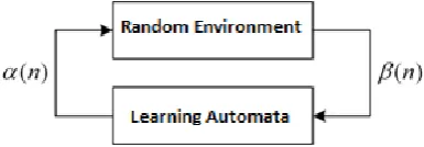
Learning automata method is to determine the optimal operation of a limited set of predefined actions which are applicable in a random environment.
An automaton transacts in a feedback circuit with environment, so in every moment the output (0)of the environment, is an input for the Automata and the action
) 0 (
decrease the probability of receiving an unfavorable response from the environment. This action is called optimal action. Figure 1 illustrates the interactive behavior of learning automata and the environment.
It should be noted that in terms of the responses which are generated by the environment, it can be considered in three different models of P, S and Q. In the P-model environment the responses are defined as a binary set including favorable and unfavorable responses (0 for favorability and 1 for unfavorable responses). For more information about learning automata the reader may refer to [16, 17].
Learning Automata can be classified into two main categories: fixed structure and variable structure learning automata (VSLA). In the first category the probability of all the actions are fixed, but the probabilities in the second category are modified in each iterations of the algorithm. A special kind of the fixed structure learning automata is called object-migration [18]. It could be considered various connections for this kind of automata which Krinisky and Krylov object-migration learning automata are two samples of them [16]. Meanwhile the fixed structure learning automata has been used for solving total weighted tardiness problem in [15]. A VSLA is a quintuple <α, β, p, T>, where α is the action set of automata, β is an environment response set, p is the probability vector, each being the probability of performing every action in the current internal automaton state, and the function of T is the reinforcement algorithm.
[image:2.595.317.532.449.633.2]In this kind of automata, if action ai is selected in step n and a favorable response is received from the environment, the probability of Pi(n) will increase and beside other probabilities related to the other actions will decrease. And for every unfavorable response received from the environment, the probability of Pi(n) will decrease and the probabilities related to the other actions will increase.
Fig. 1. Interactive behavior of learning automata and the environment
However, changes are made so that the sum of Pi(n) values always remains constant and equal to one. While receiving favorable response, the learning algorithm that is used in this paper, changes the actions probability according to the following relations in Eq. (1) and Eq. (2).
)] ( 1 [ ) ( ) 1
(n p n a p n
pi i i . (1)
i j j n p a n
pj( 1)(1 ) j( ) . (2)
And while receiving unfavorable response, changes for the actions probability will be done according to the following relations in Eq. (3) and Eq. (4).
) ( ) 1 ( ) 1
(n b p n
pi i (3)
i j j n p b r
b n
pj j
(1 ) ( )
1 ) 1
( (4)
It should be noted that in the above relations, a and b parameters are reward and penalty respectively and r represents the number of possible actions for the learning automaton. The amount of reward (a) and penalty (b) parameters values classifies automata. That is, when a=b, the automaton is called LRP. If 0<a<<b<1 the automaton is called LPεR, and if 0<b<<a<1, the automaton is called LRεP.
3.
Proposed model using VSLA
In this section we will describe how we used the VSLA to solve the SMTWT problem. In this problem, for all n jobs, n learning automata has been made which the kth automaton determines the job which will be executed in the kth location of the jobs sequence. For solving the SMTWT problem using the VSLA, the jobs are considered as actions of the automata. Then for a problem with n jobs, we will have n automaton that each of them also has n actions. As a result, each automaton will suggest one of the jobs by selecting one of its actions. At the beginning of this process, the chance of being selected is equal to all actions and total value of probability vector is equal to 1 for each automaton.
After making a solution as a result of action selection by all the automata, the proposed algorithm starts to calculate the total weighted tardiness of the solution. If the total tardiness related to the current sequence, compared to the previous iterations of the algorithm provide a smaller amount, the automata actions will be favorable and then will be rewarded. Otherwise, due to unfavorable actions selected by all n automata, they will be penalized. It is worth mentioning that in order to rewarding an action, the selection probability value related to that action is increased in the probability vector of automata, and consequently the other actions probabilities is decreased based on the learning algorithm which introduced in the previous section. In addition, to penalizing an action the scenario will be reversed.
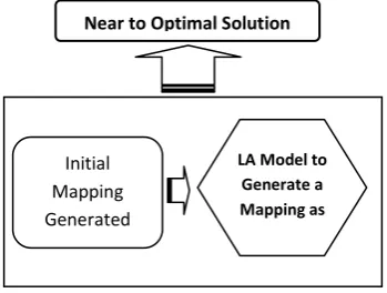
Fig. 2. The proposed model used for solving the SMTWTP using VSLA.
Figure 2 illustrates the proposed model used for solving the SMTWT problem using VSLA. As Figure 3 presents, in order to speed up search operations on the response space of the problem, learning automata algorithm is initialized using heuristic responses described in section 3.1.
[image:2.595.71.264.471.538.2]itself rapidly. The general procedure used for variable structure learning automata is presented in figure 4.
3.1 AU heuristic
One of the best heuristic search methods proposed to solve the SMTWT problem is the Apparent Urgency (AU) which has been used in many subsequent papers [19]. To use this heuristic method, first the apparent urgency AUj is calculated for all jobs as presented in Eq. (5). Then jobs are arranged in descending order of their apparent urgency.
) .
, 0 max exp( ) (
p k
p t d p
w
AU j j
j j j
(5)
Here k indicates look-ahead parameter and is adjusted by the deadline pressure; p-- is the average processing time. Furthermore, T is current time, however for static problems here is t = 0.
Fig. 3. The proposed VSLA-Scheduler model.
Creating currrent_job_order array;
initialize currrent_job_order with AU heuristic; Creating LAi for 1≤i≤number_of_jobs;
Biasing LAi to select current_job_order[i]that 1≤ i ≤ number_of_jobs;
While (w < iteration_number)
Begin
BestTWT = Total Weighted Tardiness of current_job_order;
current_job_order[i] = LAi selects its action for 1≤ i ≤ number_of_jobs; If Total Weighted Tardiness of current_job_order < BestTWT Then BestTWT = Total weighted Tardiness of current_job_order; Best_job_order=current_job_order;
Giving Reward for all LAi that 1≤ i ≤ number_of_jobs ; Else
Giving Penalty for all LAi that 1≤ i ≤ number_of_jobs; EndIf;
[image:3.595.73.248.268.400.2]End
Fig. 4. The general procedure used for variable structure learning automata.
4.
Experimental Results
In this section the datasets used for experiments has been described in detail and the comparison of the proposed algorithm with previous ones has been presented.
4.1
Simulation Environment
To evaluate the proposed model, some sample problems have been used to solve by the proposed algorithm and the other previously offered methods. These sample problems have been downloaded from the OR library [20]. The best known solutions are also available in this library [21].
There are three type of problems in term of problem size in the library (n=40, 50 and 100 jobs) that each of them involves 125 problem instances. The problem instances are generated as follows:
Each job j ( j=1,...,n ), an integer processing time pj has been assigned from the uniform distribution (1, 100), and an integer weight wj from the uniform distribution (1, 10). In order to generate different due dates for the problems, different parameters have been used. As a result, instance classes of varying hardness have been generated. The hardness of each problem depends on the range of due dates (RDD) and tardiness factor (TF). RDD refers to the relative due date and TF is delay factor for generating the problems. RDD and TF values are selected from the set {0.2, 0.4, 0.6, 0.8, 1.0} respectively. High value of RDD, indicates the wide range of due dates while the lower range of it shows a narrow range of due dates. TF value close to 1 indicates tight due date and a value close to 0 indicates a relaxed due date.
For each job j, an integer due date dj in the uniform distribution of [P(1-TF-RDD/2),P(1-TF+RDD/2)] has been assigned where P=SUM{j=1,...,n}p(j). When P(1-TF- RDD/2) is less than or equal to zero, dj is in uniform distribution (1, P(1-TF+RDD/2)). Five instances were generated for each of the 25 pairs of values of RDD and TF, yielding 125 instances for each value of n.
There are three files wt40, wt50, and wt100 in the standard library each one containing the instances of size 40, 50 and 100 respectively. Each file contains the data for 125 instances, listed one after the other. The n processing times are listed first, followed by the n weights, and finally n due dates, for each of the 125 instances.
For example in wt40 the first 40 integers in the file are the processing times for the 40 jobs in the first instance. The next 40 integers are the first instance's weights. Then 40 integers are the first instance's due dates. Finally, 40 integers are the second instance's processing times, etc.
4.2
Experiments
In this section, the results of executing the previous algorithms and the proposed algorithm (VSLA-scheduler) have been discussed for the instance problems. As discussed in previous section, there are three types of instance problems with different number of jobs which have been included in our experiments. The obtained results have been presented in comparative figures and tables. As the results shows, using learning ability of VSLA technique resulted in better solutions in contrast with the other methods considered in this paper. In tables and figures presented in this section, the results of the genetic algorithm are shown with "GA". In our tables, names "Krylov" and "Krinisky" are referring to fixed structure learning automata (FSLA) with special type of connections. It should be noted that in [16] different types of connections have been introduced for FSLA and the Krylov and Krinisky types of FSLA, have been used for solving the SMTWT problem in [15]. In addition, the word "VSLA" refers to the results of the implemented proposed algorithm to solve the problem using variable structure learning automata in the tables.
Experimental conditions were identical for all algorithms. The best parameters which have been tested previously have been used. Iterations number for all the algorithms was 5000. Rate of the crossover operator for GA was 0.8 and the rate of mutation operator was 0.3. The operators used in this algorithm had been introduced as the best ones in [14]. In LA Model to
Generate a Mapping as a solution
Initial Mapping Generated
by AU algorithm
addition the population size assumed 50 and the selection operator have been used in the algorithm was roulette wheel. The Depth of fixed structure learning automata has been considered 10 states. In the VSLA, reward (a) and penalty (b) parameters are 0.7 and 0.000015 respectively. It should be noted that the amount of the penalty parameter is considered very small in order to prevent accidental operation of automata.
The first experiment has been done to solve the 125 problems containing 40 jobs. Table 1 illustrates the results of this experiment. As noted above, for each pair of RDD and TF values, five random problems exists in the OR library. The results presented in the following tables are average of executing the algorithms for these 5 random problems. As presented in table 1, in most cases the amount of deviation percentages of the proposed VSLA algorithm is less than other algorithms. That is, the results produced by the VSLA-Scheduler are closer to the optimal values.
The second set of problems in the OR library included 50 jobs which have been used for executing second experiment. The goal of this experiment was evaluating the proposed method for the problems with more jobs. Table 2 shows the comparison of algorithms for the 125 problems containing 50 jobs. As can be seen the amount of deviation percentage, from the optimal solution, related to the values generated by the proposed algorithm is lower than the results of other algorithms.
Table1: deviation percentages Comparison for different algorithms about problems containing 40 jobs
VSLA GA Krinsky Krylov TF RDD 13.075 21.393 6.894 83.174 0.2
0.2 2.648 13.209 5.401 3.557 0.4 2.961 10.155 4.724 3.703 0.6 1.039 5.628 4.618 7.607 0.8 0.211 4.692 3.396 5.804 1 46.386 47.590 93.976 292.169 0.2
0.4 5.785 34.399 4.394 33.257 0.4 4.590 19.894 11.061 15.267 0.6 1.648 5.916 6.190 8.009 0.8 0.278 4.427 6.570 5.840 1
- - - - 0.2 0.6 17.381 110.551 23.858 111.901 0.4
4.890 38.963 9.566 30.072 0.6 1.403 9.605 3.703 4.776 0.8 0.599 9.618 3.792 6.657 1
- - - - 0.2 0.8 48.901 447.719 59.206 283.131 0.4
5.227 56.392 12.376 37.938 0.6 1.965 15.243 4.566 9.179 0.8 0.337 2.884 2.803 2.351 1
- - - - 0.2 1 21.240 171.525 8.088 393.592 0.4
4.734 22.467 8.613 14.592 0.6 1.665 13.446 3.633 4.177 0.8 0.655 5.423 4.942 4.688 1 1.364 9.980 4.946 8.474 Average
Table2: Comparison of deviation percentages related to different algorithms for problems containing 50 jobs.
VSLA GA Krinsky Krylov TF RDD 3.296 15.025 3.644 28.392 0.2
0.2 5.465 10.841 4.017 7.004 0.4 4.019 5.174 3.425 5.298 0.6 1.507 3.530 5.840 6.518 0.8 0.175 1.625 4.210 4.686 1 22.562 141.723 78.685 994.558 0.2
0.4 9.420 41.377 6.221 49.665 0.4 6.384 15.912 9.442 17.104 0.6 1.055 9.474 7.344 9.263 0.8 0.170 2.844 2.824 3.967 1
- - - - 0.2 0.6 16.769 154.882 20.796 96.422 0.4
6.531 39.691 14.282 32.612 0.6 1.125 6.208 5.330 10.214 0.8 0.592 3.306 5.020 6.003 1
- - - - 0.2 0.8 17.452 120.591 24.407 111.017 0.4
7.431 26.216 8.634 19.781 0.6 1.992 9.719 4.895 14.098 0.8 0.503 2.573 4.955 5.219 1
- - - - 0.2 1 19.495 122.257 34.011 126.628 0.4
6.295 44.049 11.053 23.024 0.6 1.189 10.909 3.402 4.776 0.8 0.709 3.500 3.362 4.294 1 1.485 7.455 5.121 8.584 Average
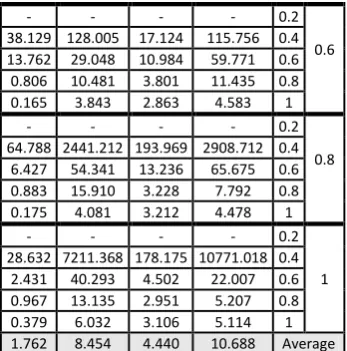
Table 3 shows the comparison of algorithms for the 125 problems containing 100 jobs. Values generated by the proposed algorithm in this table are also lower than the results of other algorithms. The table shows that by increasing the number of jobs in the problems, there is a meaningful difference between the results of proposed algorithm and the other ones.
Finally, as the achieved results from the all three experiments summarized in figure 5, the results illustrate that the proposed algorithm (VSLA-Scheduler) gives minimum deviation percentages from the optimal results in contrast with the other previously presented algorithm which was studied in this paper.
5.
Conclusion
In this paper, a scheduling method based on learning automata technique has been presented for solving the single machine total weighted tardiness problem. In order to evaluate the proposed method, some of previous methods for solving this problem have been simulated and their results compared with the proposed algorithm's results.
The simulated algorithms include two kinds of the FSLA and a GA approach. The comparisons have showed that the variable structure of learning automata have better performance than fixed structure for solving the SMTWT problem.
method compared to existing ones is using a learning system based on the environmental feedback. That is, each time producing a new solution, the VSLA-scheduler algorithm updates the probability vector of the set of automata according to the amount of performance metric (TWT) achieved by the solution.
Genetic algorithms have a random nature and this feature probably diverge it from appropriate solutions. The proposed method with the use of learning ability and correction of previous changes by rewarding and penalizing the automata has the ability to generate better results
Table3: Comparison of deviation percentages related to different algorithms for problems containing 100 jobs.
VSLA GA Krinsky Krylov TF RDD 12.471 26.285 6.082 29.762 0.2
0.2 19.205 10.283 2.988 10.045 0.4
9.401 4.812 3.660 8.860 0.6 1.635 2.773 5.601 8.243 0.8 0.154 1.292 3.597 5.363 1 64.770 461.029 41.465 2843.570 0.2
0.4 25.276 38.946 7.504 37.398 0.4
9.306 14.709 8.559 21.911 0.6 0.797 4.753 7.238 11.300 0.8 0.186 1.747 5.033 5.400 1
- - - - 0.2 0.6 38.129 128.005 17.124 115.756 0.4 13.762 29.048 10.984 59.771 0.6 0.806 10.481 3.801 11.435 0.8 0.165 3.843 2.863 4.583 1
- - - - 0.2 0.8 64.788 2441.212 193.969 2908.712 0.4
6.427 54.341 13.236 65.675 0.6 0.883 15.910 3.228 7.792 0.8 0.175 4.081 3.212 4.478 1
- - - - 0.2 1 28.632 7211.368 178.175 10771.018 0.4
[image:5.595.342.516.71.247.2]2.431 40.293 4.502 22.007 0.6 0.967 13.135 2.951 5.207 0.8 0.379 6.032 3.106 5.114 1 1.762 8.454 4.440 10.688 Average
Fig. 5. Average of deviations percentage from the best known solutions.
6.
ACKNOWLEDGMENTS
The work presented in this paper is supported by Research Center of Islamic Azad University, Sofian branch in Iran.
7.
REFERENCES
[1] Lenstra, J.K. Kinnooy Kan, A. H. G. and Brucker, P. 1977. Complexity of machine scheduling problems. Annals of Discrete Mathematics. 1. 343–362.
[2] Madureira, A. Ramos, C. and Silva, S. 2001. A GA based scheduling system for dynamic single machine problem. In Proceedings of the 4th IEEE International Symposium
on Assembly and Task Planning Soft Research Park. 262–267.
[3] Morton, T. E. David, P. W. 1993 Heuristic Scheduling Systems. John Wiley & Sons.
[4] Baker, K.R. 1974 Introduction to Sequencing and Scheduling. Wiley. New York.
[5] Lawer, E.L. 1977. A pseudopolinomial algorithm for Sequencing Jobs to Minimize Total Tardiness. Annals of Discrete Mathematics. 331–342.
Total WT Scheduling Problem. Discrete Applied Mathematics. 26. 235–253.
[7] Potts, N. Van Wassenhove, L. N. 1991. Single Machine Tardiness Sequencing Heuristics. IIE Transactions. 23. no. 4. 346–354.
[8] Shwimer, J. 1972. On the n-job, one-machine, sequence independent scheduling problem with tardiness penalties: a branch-bound solution. Management Science. 18. no. 6. 301–313.
[9] Rinnooy Kan, H.G. Lageweg, B.J. and Lenstra, J.K. 1975. Minimizing total costs in one-machine scheduling. Operations research. 23. no. 5. 908–927.
[10]Potts, C.N. Wassenhove, L.N.V. 1985. A branch and bound algorithm for the total weighted tardiness problems. Operations Research. 33. no. 2. 363–377. [11]Schrage, L. Baker, K.R. 1978. Dynamic programming
solution of sequencing problem with precedence constraints. Operations research. 26. 444–449.
[12]Huegler, P. A. Vasko, F. J. 1997. A performance comparison of heuristics for the total weighted tardiness problem. Computers & Industrial Engineering. 32. no. 4 753–767.
[13]Crauwels, H.A.J. Potts C.N. and Wassenhove, L.N.V. 1998. Local search heuristics for the single machine total weighted tardiness scheduling problem. INFORMS Journal on Computing. 10. no. 3. 341–350.
[14]Ferrolho, A. Crisóstomo, M. 2007. Single Machine Total Weighted Tardiness Problem with Genetic Algorithms.
In Proceedings of the 3rd International Conference on Computer Systems and Applications. Amman.1–8. [15]Asghari, K. and Meybodi, M. R. 2009. Solving Single
Machine Total Weighted Tardiness Scheduling Problem using Learning Automata and Combination of it with Genetic Algorithm. In Proceedings of the 3rd Iran Data Mining Conference. Tehran University of Science and Technology. Iran.
[16]Narendra, K. S. Thathachar, M. A. L. 1989. Learning Automata: An Introduction. Prentice-hall. Englewood cliffs.
[17]Najim, K. Poznyak, A. S. 1994. Learning Automata: Theory and Application. Tarrytown. Elsevier.
[18]Oommen J. and Ma, D. C. Y. 1998. Deterministic Learning Automata Solutions to the equipartitioning problem. IEEE Transactions on Computers. 37. 2-13. [19]Morton, T.E. Rachamadugu, R.M. and Vepsalainen, A.
1984. Accurate myopic heuristics for tardiness scheduling. GSIA Working Paper. no. 36. Carnegie-Mellon University. PA. 83-84.