Hybrid Model for Location Privacy in Wireless Ad-Hoc
Networks for Mobile Applications
B. N. Jagdale
Department of Information Technology, MIT College Of Engineering, Pune-411038,
Maharashtra
N. S. Gawande
Department of Information Technology, MIT College Of Engineering, Pune-411038,
Maharashtra
ABSTRACT
A wireless ad-hoc network is a decentralized type of wireless network. The network is ad hoc because it does not rely on a preexisting infrastructure, such as routers in wired networks or access points in managed (infrastructure) wireless networks. Now a day in fast growing world, use of internet is increasing popularly and at the same time Location-based service is also getting more popular even in ad-hoc network. Location-based service providers require user’s current locations to answer their location-based queries. The primary objective of the present work is to develop a system which preserves the location privacy of the concerned individual by applying K- anonymization and obfuscation algorithms . This objective is achieved by simulating K- anonymization and obfuscation algorithms for Manhattan mobility model and Waypoint mobility model using NS-2.34 environment. In the experiments, the user’s current location is hide by rectangle [bounding box] according to users privacy need.
General Terms
Ad-hoc Networks, Security, Algorithms
Keywords
Location-based service [LBS], wireless ad-hoc networks, LCA, GCA.
1.
INTRODUCTION
Location Based Services is defined as the ability to locate a mobile user geographically and deliver services to the user based on his location. The location based services means that “the services that integrate a mobile device’s location or position with other information so as to provide added value to the user”. So knowing your location or how far you are from a specific location would not be valuable by itself. Only if it can be related to other location this gives it meaning and value. LBS has a variety of applications that can be offered to organizations such as government, emergency services, commercial and industrial organizations for example, breaking news, traffic information, tracking and way finding. As LBS has the ability to locate a mobile user geographically. It threatens the privacy and the security of the users. A decentralized approach introduce in [1] to the location privacy that combines k-anonymity with obfuscation, which enable agents to act on the behalf of peers requiring a location-based service. As a result it does not requires to trust on any involved party, neither its peers not the LSP. There are no restrictions for the agents’ positions: they could be located in a street, an office building, a shopping mall, or public place. Whereas as per [2] framework has two main components, the location anonymizer and the privacy-aware query processor. The location anonymizer acts as a third trusted party that blurs the exact location information of each user into a cloaked
designer to find the optimal location-privacy preserving mechanism [LPPM] for LBS given each user’s service quality constraints against an adversary implementing the optimal inference algorithm. Hence in this research work based on such location privacy preferences, a new solution, based on obfuscation techniques, which permits to achieve, and quantitatively estimate through a metric, different degrees of location privacy for mobile applications is proposed.
2.
PROBLEM FORMULATION
In the present world, use of internet is a major source of data. User data and other vital data flows through the internet. This data is prone to be misused by external entities. Even though there are several policies to prevent data misuse, these aren’t foolproof. Hence this work aims to hide the data that is vital to preserve the privacy of any user. The proposed system uses k-anonymity and obfuscation concept to achieve this task. Hence based on extensive literature survey the problem is formulated as below:
Given a set of nodes n1, n2,. . . , nn with LCA a1, a2, . . . ,
an, respectively, a set of moving objects m1, m2, . . . , mm,
and a required anonymity level k and obfuscation area O , we find LCA and GCA an aggregate location for each node ni in the form of Ri = (Ai, Ni ), where Ai is a
rectangular area containing the GCA area of node Ai
and Ni is the number of node residing in the GCA areas
of the nodes in Ai, such that Ni ≥ k.
3.
K-ANONYMITY AND
OBFUSCATI-ON STRATEGY
In wireless ad-hoc network obfuscation make’s communication confusing by hiding node current position in minimum bounding box known as locally cloak area [LCA] at the same time k-anonymity make node position undistinguishable in group of [k-1] users using GCA algorithm.
3.1
Generating the LCA
Locally cloak area is computed to achieve obfuscation in which small bounding box is developed by forming the LCA of the query initiator via some constants such as
The constant c which will determines the ratio between the width and the length of the LCA.
The constants c1 and c2 determine the minimum and
maximum distance of the agent’s position from the boundary of its LCA.
If an agent A’ provides its LCA to an agent A and some part of its LCA lies outside the communication range of agent A, then agent A can easily render a more precise location of A’. Restricting the position of A’ via c1 and c2 to a smaller
rectangle in the LCA ensures a larger obfuscated area for A’.
3.2
Generating the GCA
To compute the GCA for an agent ‘j’, assumed that ‘k’ is the desired anonymity level of ‘j’ and ‘n’ is the number of LCAs reported by its neighbors. For the computation of the GCA, we need to find the smallest rectangle ‘r’ that encloses a k-subset (including j’s LCA) from the ‘n’ reported LCAs. The LCA of an agent ‘i’ is described by (xmini, xmaxi, ymini, ymaxi).
The algorithm removes at each iteration one rectangle of the ‘n’ rectangles excluding the agent’s rectangle rj. Each removal
of a rectangle minimizes the size of the GCA. The algorithm continues until the number of remaining LCAs is equal to ‘k’.
Algorithm 1. Find GCA
Input : A set R of LCAs, given by (xmini , xmaxi , ymini , ymaxi ), an anonymity level k, the agent j.
Output: A rectangle that covers k LCAs including the LCA of the agent j.
1.1 Sort the lists xmini , ymini in increasing order, the lists xmaxi , ymaxi in decreasing order;
1.2 while |R| > k do
1.3 Calculate m(xmin), m(xmax), m(ymin), and m(ymax); 1.4 Find the minimum from m(xmin), m(ymin) and maximum from m(xmax), and m(ymax);
1.5 Delete the LCA from R which has the maximum value; 1.6 returns a minimum rectangle covering the LCAs in R that are not eliminated;
4.
METHODOLOGY
The Wireless ad-hoc networks are an emerging technology which finds variety of applications in military, movement tracking, industries and medical fields. Wireless ad-hoc networks are self configurable, self healing networks. Considering this need in this work two mobility models are used in the simulations as mentioned below:
Manhattan Model
Waypoint Model
The Manhattan mobility model uses a grid road topology. This model is mainly proposed for the movement in urban area, where the streets are in an organized manner and the mobile nodes are allowed to move only in horizontal or vertical direction. At each intersection of a horizontal and a vertical street, the mobile node can turn left, right or go straight with certain probability. The parameter setting for Manhattan mobility model is as shown below.
Simple waypoint [pathway] model is a way to integrate geographic constraints into the mobility model and the node movement to the pathways in the map. The map is predefined in the simulation field. This graph can be either randomly generated or carefully defined based on certain map of a real city. The vertices of the graph represent the buildings of the city and the edges model of the streets and freeways between those buildings. Initially, the nodes are placed randomly on the edge. Then for each node a destination is randomly chosen and the node moves towards this destination through the shortest path along the edges. Upon arrival, the node pauses for ‘T’ pause time and again chooses a new destination for the next movement. This procedure is repeated until the end of simulation. However, since the destination of each motion phase is randomly chosen, a certain level of randomness still exists for this model. So, in this graph based mobility model, the nodes are traveling in a pseudo-random fashion on the pathways.
4.1
Implementation
and
Performance
Analysis
rectangle and the rectangles of k − 1 other nodes in wireless ad hoc network, thus can achieve location privacy for secure communication. Our proposed approach reveals as little information as possible.
[image:3.595.314.545.80.273.2]The system architecture design for the proposed system is as shown in the Fig.1. System architecture shown in Fig.1 is executed by using simulation environment NS-2.34. To run simulation; topology set up is done using tcl script. The tcl file intern called all the .cc files NS-2.34. The LCA Algorithm is implemented in NS2 core .cc files such as location. h, mobile node .cc, mobile node .h where as GCA algorithm is implemented using tcl script.
Fig 1: A System Architecture Design
4.2
Modifications to NS2.34
In wireless ad-hoc network obfuscation make communication confusing by hiding node current position in minimum bounding box known as locally cloak area [LCA], to perform this implementation, it is essential to add some important patches in NS-2.34 core files such as:
ns-allinone-2.34/ns- 34/common/mobilenode.cc, mobilenode.h
ns-allinone-2.34/ns-2.34/common/location.h
ns-allinone-2.34/ns-2.34/trace/ cmu-trace.cc , cmutrace.h
ns-allinone-2.34/ns-2.34/tcl/lib/ns-default.tcl, nsmobilenode.tcl.
4.3
Setup in NS-2.34 Simulation
The scenario to simulate and GCA algorithm computation are defined in simulation.
1. Create the simulator object 2. Setup the network nodes 3. Setup the routing mechanism 4. Create transport connections 5. Setup user applications
6. Schedule LCA request transmission for GCA computation.
7. Stop the simulation
4.4
Experiment Setup
To setup experiment for LCA and GCA, two mobility models as Manhattan and Waypoint Models are used in the simulations of wireless ad-hoc network with AODV and Dump agent protocol.
A. Manhattan Model:
[image:3.595.59.276.213.346.2] [image:3.595.317.539.493.670.2]The parameter setting for Manhattan model is as shown in Table 1.
Table 1. NS2 Simulation Parameters
Parameter name Value
Area of Sensor Field 500×500
Channel Channel/Wireless Channel
Topology Used Random
Number of Sensor Nodes for
the simulation 70
IPQ length 64
Transmissions Range 0.1 Interface Range 0.1
MAC protocol Mac/802_11Ext Routing Protocol AODV DumpAgent Max Sensor node 5, 10 ,15, ……… 70
Sink Node All
k- anonymity level 5 , 10 ,15, 20 , 25 LCA and Obfuscation Area 500 m2
4.4.1
Manhattan Mobility Model Scenario used
for Simulation
Manhattan Mobility model scenario implemented in NS2.34 simulation is as shown in Fig. 2.The Manhattan mobility model scenario as shown in Fig. 2 used for the simulation is created, which shows that the topology used for it is Random topology with 70 nodes deployed in the sensor field of 500×500 area. The different properties of the sensor node are as shown in Table1. Here we assume that there are 5 source nodes (max. up to 70) are randomly selected that generates the events at random time interval (0 to 120 sec). According to the parameter setting of source node (uniformly random node) will generate LCA request which will be broadcast at random time towards the Sink Nodes and these packets are forwarded by the cooperative nodes in the network as per routing table and path defined by AODV, Dumb Agent protocol and MAC 802_11EXT protocol . The source node that needs to find GCA will send LCA query request to the sink nodes. According to parameter setting source node can set different k- anonymity level as well as obfuscations area.
Fig. 2: Screen shot of Manhattan Mobility Model scenario
4.4.2
Results and Graphs of Manhattan Model:
Dump Agent Routing: LCA Computation Result
Sender.tr Manhattan Model Waypoint Model MobilityModel Simulation GCA Algorithm LCAAlgorithm
Routing Protocol DumbAgent, AODV
Fig. 3: LCA Computation Result for sender in Manhattan mobility model using Dump Agent Routing
[image:4.595.83.523.412.721.2] Receiver.tr
Fig. 5: GCA Computation Result for receiver in Manhattan mobility model using Dump Agent Routing
Fig. 6: GCA Computation Result for receiver in Manhattan mobility model using AODV Routing
Fig. 3 shows the screen shot of LCA Computation result for sender node in Manhattan mobility model using Dump Agent Routing which generated by running tcl script using NS2.34. Fig. 4 shows the screen shot of LCA Computation result for receiver node in Manhattan mobility model using Dump Agent Routing generated by running tcl script using NS2.34.
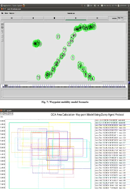
Fig. 7: Waypoint mobility model Scenario
Fig. 9 : Screen shot of GCA Computation Result for receiver in waypoint mobility model using AODV Routing
[image:7.595.85.512.475.690.2]Fig. 11 : GCA Computation Result of Average GCA Area for sender node in Manhattan mobility mode
[image:8.595.75.524.518.739.2]4.4.3
GCA Computation Result
Fig. 5 shows the screen shot of GCA Computation result for Sender Node ‘19’ in Manhattan mobility model using Dump Agent Routing. Fig.5 shows the result of GCA computation when node id ‘19’ request LCA to its neighbors. GCA of node id’19’ is shown in red color, whereas the result of LCA computation for node id ‘19’ is shown in bottle green color.
4.4.4
AODV Routing
The similar results are obtained with AODV Routing protocol for LCA, whereas the GCA Computation varies for time required for the processing as shown in Fig. 6. Fig. 6 shows the result of GCA computation when node id ‘17’ request LCA to its neighbors. GCA of node id ‘17’ is shown in red color, where as the result of LCA computation for node id ‘17’ is shown in green color. From Fig. 5 and Fig. 6 it is observed that, when sender as well as sink used to communicate each other node in a wireless ad hoc network masks its current position by providing a rectangle instead of a point as its location.
B. Waypoint Model
The parameter setting for Way point Model is as shown in Table 2.
Table2. Ns2 Simulation Parameters
Parameter name Value
Area of Sensor Field 500×500
Channel Channel/Wireless Channel
Topology Used Random
No. of Sensor Nodes for the
simulation 76
Packet Length 50
IPQ length 64
Transmissions Range 0.1
Interface Range 0.1
MAC protocol Mac/802_11Ext
Routing Protocol AODV Dump Agent Max Sensor node 5, 10 ,15, ……70
Sink Node All
k- anonymity level 5 , 10 ,15, 20 , 25 LCA and Obfuscation Area 500 m2
4.4.5
Waypoint Mobility Model Simulation
Scenario
Waypoint Mobility model scenario implemented in NS2.34 simulation is as shown in Fig. 7.
The Waypoint mobility model scenario as shown in Fig. 7 used for the simulation is created, which shows that the topology used for it is Random topology with 76 nodes deployed in the sensor field of 500×500 area. The different properties of the sensor node are as shown in Table 2. Here we assume that there are 5 source nodes Here we assume that there are 5 source nodes (max. up to 76) are randomly selected that generates the events at random time interval (0 to 120 sec). According to the parameter setting of source node (uniformly random node) will generate LCA request which will be broadcast at random time towards the Sink Nodes and these packets are forwarded by the cooperative nodes in the network as per routing table and path defined by AODV, Dumb Agent protocol and MAC 802_11EXT protocol . When source node need to find GCA, node will send LCA query request to the sink nodes. According to parameter setting
source node can set different k- anonymity level as well as obfuscations area.
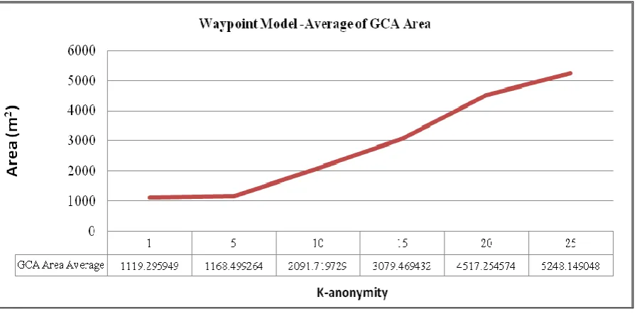
Fig. 8 shows the result of GCA computation when node id ‘66’ request LCA to its neighbors. GCA of node id ‘66’ is shown in red color, whereas the result of LCA computation for node id ‘66’ is shown in green color. Fig. 9 shows the result of GCA computation when node id ‘15’ request LCA to its neighbors. GCA of node id ’15’ is shown in red color, whereas the result of LCA computation for node id ‘15’ is shown in green color.
[image:9.595.51.283.337.547.2]4.4.6
Effect of K & density on GCA Computation
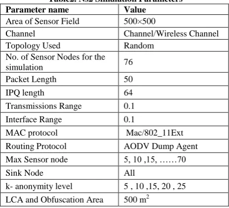
Fig. 10 and Fig. 11 shows the effect GCA computation result and average GCA area for sender node in Manhattan mobility model for k- anonymity value 1, 5, 10, 15, 20. From the simulation result is seen that more the node density, the GCA algorithm maximizes the bounding box size, which results in maximum location privacy for secure communication. From simulation results as shown in Fig. 12 and Fig. 13 it is seen that more the node density, the GCA algorithm maximizes the bounding box size, which results in maximum location privacy for secure communication. Again from Fig. 13 it is observed that as value of ‘k’ anonymity increases from 15 to 25, then GCA area also increases up to certain level for k.5. CONCLUSION
This work present an approach that combines obfuscation and anonymization to ensure both location and anonymity privacy for mobile agents. This approach does not require any central trusted party for computation of obfuscation and anonymization method results which can be further used for LBS request. Form simulation in NS2.3 is seen that the obfuscation and anonymization approach provides the best method of cloaking depending on the mobile user privacy. From simulation it is seen that when sender and receiver communicate in a clique obfuscates (masks) its current position by providing a bounded box instead of a point as its location. During simulation it is seen that GCA algorithm generates minimum bounding box of size LCA. Again it is seen that more the node density, the GCA algorithm maximizes the bounding box size, which results in maximum location privacy for secure communication. The value of ‘k’ anonymity increases then GCA area also incases up to certain level.
5.
ACKNOWLEDGMENTS
Authors would like thank the Principal of MIT college of Engineering, Pune-38 for cooperation and providing well equip laboratory. Again thanks due to the Prof. V. V. Deshpande for his full hearten cooperation and critical review during progress of project work. We thank to the experts who have contributed towards the development of this research article.
6.
REFERENCES
[1] T. Hashem and L. Kulik , 2007, “Safeguarding Location Privacy in Wireless Ad-Hoc Networks” , UbiComp 2007, LNCS 4717, pp.372–390, Springer-Verlag Berlin Heidelberg .
[2] M. F. Mokbel, C. Y. Chow and W. G. Aref , 2009, “The New Casper: Query Processing for Location Services without Compromising Privacy’, VLDB Endowment, ACM 159593385-9/06/09.
Wireless Sensor Networks”, IEEE Mobile Computing, vol.10, no.1, pp.1-14.
[4] M. Duckham and L. Kulik, 2005, “A Formal Model of Obfuscation and Negotiation for Location Privacy”, Proc. Of Pervasive Computing, 2005: pp.152–170. [5] L. Sweeney and P. Samarati, 2002, “Protecting Privacy
When Disclosing Information: k-anonymity & its enforcement through Generalization”, in Proc. of MobiCom.
[6] L. Sweeney, 2002, “k- Anonymity: A Model for Protecting Privacy.” International Journal on Uncertainty, Fuzziness and Knowledge-based Systems, vol. 10, no.5, pp.557-570.
[7] M. Duckham and L. Kulik, 2007, “Location Privacy & Location Aware Computing”, in Proceedings of HICSS, pp.1-7.
[8] Y. Zhu and R. Bellati, 2007, “Compromising Location Privacy in WSN with limited information”, Proc. of ICDCS-2007, Pages 24.
[9] C. A. Ardagna, M. Cremonini, E. Damiani, S. De, C. Vimercati, and P. Samarati, 2007, “Location privacy protection through obfuscation-based techniques”, Lecture Notes in Computer Science, LNCS 4602, Springer, Berlin, pp.47–60.
[10] M. Duckham and L. Kulik., 2007, “Location Privacy & Location Aware Computing” Proceeding of HICSS, pp.213-220.
[11] R. Shokri, G. Theodorakopoulos , C. Troncoso, J. Hubaux and J. Boudec, 2012, “Protecting Location Privacy: Optimal Strategy against Localization Attacks”, Proceedings of CCS’12, October 16–18, 2012, Raleigh,