A Parallel Algorithm to Calculate the Cost rank of a
Network
Thaier Hamid
University of Bedfordshire, UKCarsten Maple
University of Bedfordshire, UKYong Yue
University of Bedfordshire, UK
ABSTRACT
We developed analogous parallel algorithms to implement CostRank for distributed memory parallel computers using multi processors. Our intent is to make CostRank calculations for the growing number of hosts in a fast and a scalable way. In the same way we intent to secure large scale networks that require fast and reliable computing to calculate the ranking of enormous graphs with thousands of vertices (states) and millions or arcs (links). In our proposed approach we focus on a parallel CostRank computational architecture on a cluster of PCs networked via Gigabit Ethernet LAN to evaluate the performance and scalability of our implementation. In particular, a partitioning of input data, graph files, and ranking vectors with load balancing technique can improve the runtime and scalability of large-scale parallel computations. An application case study of analogous Cost Rank computation is presented. Applying parallel environment models for one-dimensional sparse matrix partitioning on a modified research page, results in a significant reduction in communication overhead and in per-iteration runtime.We provide an analytical discussion of analogous algorithms performance in terms of I/O and synchronization cost, as well as of memory usage.
General Terms
Security, Algorithms, Networking.
Keywords
Parallel computing, distributed algorithms, PageRank..
1.
INTRODUCTION
The CostRank algorithm is used as cost-centric model checking for network security. It uses an iterative numerical method to compute the maximal eigenvector of a transition matrix with the hosts‟ cost value derived from designated files structures. The principal indication for the CostRank algorithm to be considered a state is important if other important states are linked to it. However, not all states are equal in importance. The link from different states holds different cost value [5]. For n states V=v; v = 1; 2;. . .; n the corresponding CostRank is set to ; v = 1; 2 ……; n. The mathematical formulation for the recursively defined CostRank is presented in the following equations:
d u Bv u u v
N d i
v( 1) 1 ( )*( , )
Where v is an initial state.
v
(i1)(
v
)
d
uBv
(u)*
(u,v)OtherwiseTo get the normalized cost matrix we used the following formula:
Ov
w c u w
v u c v u
) , ( )
, ( ) , (
Whereof
out
(
u
)
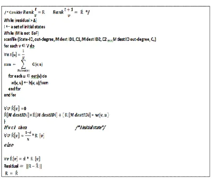
[image:1.595.316.535.331.522.2]Since this is a recursive formula, an implementation needs to be iterative and will require several iterations before stabilizing to an acceptable solution. This can be solved in an iterative fashion using algorithm thus:Let the probability of intrusion of attack be state v at time t and d be a damping factor representing the probability of an attacker to continue penetrating the current path of the attack..
Figure-1: Serial CostRank Algorithm
The initial value vector is calculated by following this formula: 1/V; where V is the number of states present that describes the initial CostRank value for all states Vi. Then the excursive formula is iterated until two consecutively iterated CostRank vectors are similar enough [5].The CostRank computational algorithm we proposed in this paper does not directly take the input from link files; instead, we converted the out-link file into a binary graph file structure M as illustrated in Figure 2. The total number of floating point numbers read from personalization file is |Ѵ| at the start of an execution. While the size of the data read from the graph file during iteration is 2* |É| +2*|Ѵ| integers. Towards the end of the execution, total |Ѵ| floating point numbers representing the consequential CostRank vectors are cast off into disks. Therefore, the total is:
|| V | 2* | É | 2 | * | | *
2
V18 nearly constant, the total time spent on disk I/O during an
[image:2.595.54.288.100.276.2]execution is O(n) where n = |Ѵ|.
[image:2.595.326.542.126.232.2]Figure-2: The structure of a sample graph file
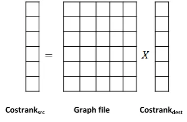
Figure 2 shows the structure of a graph file. This file consists of a file header and states entries for the hosts in the graph. The file header has three components: total number of states (v), total number of links (m) and the maximum out -degree in the graph. A state entry stores the necessary structural information for a host. It consists of a state ID, the out-degree, and the three forward links (Link 1, Link 2, and Link n) along with corresponding cost for each link (C1, C2, and Cv) respectively. The list is an array of d state IDs. All numbers are stored in 4 byte integers.The total volume of the graph file is = 4*(3+2v+2m). An example of representing states to graph file is shown in figure 2. As to memory usage, we used a buffer to hold personalization vector, size of 4 * max. out-degree. The setup for the CostRank implementation is done by creating two arrays of floating point values representing the rank vectors as you can see in figure 3, called the Costranksrc and the Costrankdest. Each rank vector has V
entries, where V is the total number of states in the graph file.
Figure-3: The setup for the CostRank implementation [7].
For each iteration step, the Costranksrc is referred to the rank
score of iteration i and the Costrankdest is referred to the rank
score of iteration i + 1. The sequential version of the CostRank computation is shown in figure 1.
2.
ANALOGOUS COST RANK
ALGORITHM
We developed a parallel algorithm to implement CostRank for distributed memory parallel computers using multi processors. We selected parallel in-memory (Piccolo) algorithms [14] to extensively reduce access share state stored in memory and
iterations, which include table partitioning (local access), synchronization of distributed table, check point/restore and load balance/ and task scheduling.
Figure-4 synchronization of distributed binary graph files
Our aim is to make CostRank calculations for the growing number of hosts in a fast and a scalable way. An accurate and efficient computing of the CostRank scores for a large network has to be addressed in order to secure significant assists among huge number of hosts in the network.The performance of serial algorithms is limited because these algorithms can only run on a single processor. Implementing the CostRank-calculations in a parallel environment opens several possibilities in partitioning the data and the load balancing the data. When we tried to implement partitions with load balance, we divided the binary graph file to relevant uniform parts and distributed to different hosts participating in rank calculating. This move lead to efficient use of all processors and this improved the overall quality of computing.We have considered three different methods for partitioning [11] the state matrix among the Processors thus:
1-Divide the matrix using a row-wise distribution 2-Divide the matrix using a column-wise distribution
3-Divide the matrix as a 2D grid
The method chosen for our computations is the row-wise partitioning. We employed the cluster computing technology. We first equally partitioned the binary graph file M into β files, named later Mi, where 0 ≤ i < β, and allocated each partition to a PC processor. At each processor, we allocated additional array of floating point Vi in main memory for portion of rank vector, having β N entries to represent the portion of the corresponding source rank vector; and created a synchronization file Si, storing pairs of destination state ID and their corresponding rank scores, called the “synch”, to represent the destination rank vector adopted from the Serial CostRank Algorithm. We first partitioned the binary link structure file M into β portions M0, M1, .. ,Mβ−1, such that each Mi started from ( * 1)
Vi to
) * ) 1 ( (
V
i .
In other words, the outgoing links of a node are bucketed according to the range that the identifier of the destination page falls into. We also created following arrays of Costrankdest, i, out-vector, and Costranksrc, i for each PC. The
Costrankdest, i array and the out-vector array contain only the
corresponding Vβ entries, while the Costranksrc, i array
contains the full set of rank scores that each machine needs to compute in each iteration step. The parallel version of the CostRank computation is shown in Figure 5.Suppose Vβ receives an update message from some foreign document, and supposeXVβ1 and XVβ2 are two documents local to XVβ, both
of which are out linked by XVβ then, one method of update
[image:2.595.66.257.490.614.2]would be to simply increment the CostRanks of XVβ1 and
XVβ2by w(v, u) ← h(v, u)/sum ×(update message received
from XVβ). If the absolute change in CostRank were to
exceed epsilon, then XVβ1 would send its own local update
message to XVβ2 this message would trigger a further update
in the CostRank of XVβ2. In sum, the idea would be to set-up a
[image:3.595.57.279.151.313.2]local messaging analogue between foreign linked documents.
[image:3.595.317.541.223.362.2]Figure-5 Parallel CostRank Algorithm
Figure 6 shows the parallel CostRank computation during an iteration using 10 processors and extra 2 pcs to perform synchronizations of Synch files between processors.
Figure-6 Matlab Topology Structure
3.
IMPLEMENTATION OF PARALLEL
COSTRANK ALGORITHM AND
RESULTS
3.1
Matlab Topology Setup
We did experiments on a cluster of 12 computers built with Pentium Core2Duo 2.54Ghz processor, 2GB RAM, 250GB Hard Disk interconnected with Gigabit Ethernet LAN, running the Linux operating system. We created a graph file containing 28 903 states, with about 1.2 million links. This are stored in sparse format including the cost values and other fields in our graph file it totaled up to 74.6MB in CRS format.Variable Si corresponds to the synch file; Mi to the partitioned binary graph structure file; and Vi to the portion of source rank vector in memory residing at processor i. During iteration, the following process occurred: first, computing a new rank based on corresponding part of graph file Mi then pushing the calculated values in to Costrankdest vector. These processes will continue until the residual value exceeds epsilon. The calculated rank Costrankdest will be added to the local updated queue if the out link is local, or if the outlink belongs to a foreign host, it is sent to the master host.
3.2
I/O cost
During iteration, each processor has to do the following functions: read the portion of Mi, compute the destination rank scores, write a created synch file Si back to disk and then re-read the Si during synchronization. Thus the total read-write I/O cost will be:
i o
i paralell Mi Si Qi
C
0
/ | | 2| |
Q S M
| | 2| |
Where Qi =local update queue. At this time, the outline of all β partitions of Mi is equal to the binary graph structure file M, and the summation of all packet files Si is S.
0 1 2 3 4 5 6 7 8 9
6 8 12 15 17
N
o.
of
pr
oc
e
ss
or
s
Data Access(GB)
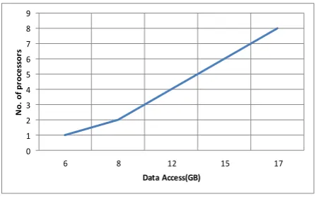
Figure 7: I/O cost during iteration.
The performance measure for parallel I/O is based upon an evaluation of its possible data movement and iterations. This data transfer rate is dependent upon the communication bandwidth of each processing element and I/O device, and on the collective start-up latency for the complete transfer.Following our analysis mentioned above, the I/O cost of data access is increased by the factor of 2 x Si and local update queue Qi that explain the incremental of I/O with the number of processors as we can see in figure 7.
3.3
Memory Norm
All processors have to assign fixed size of memory to fit an array of source rank vector Vi. Therefore, the total memory usage will be:
V Vi paralell
CMem | |
[image:3.595.57.273.379.496.2]As the source rank vector V is divided into β portions, the outline of all portions Vi will be equal to the size of the source rank vector V. Figure 8 reports the total memory usage during computation.
Figure-8 Memory Usage
0 50 100 150 200 250 300
1 2 4 6 8 10
M
em
or
y
Us
ag
e
(M
B
)
[image:3.595.318.544.593.718.2]20 As seen in figure 8, there is an increase in memory usage
when only two processors were used. This is due to the extra storage needed for synchronized files. As the number of processors increased with distributions of the tasks, the total memory usage decreased as in 4, 6, 8 and 10 processors.
3.4
Synchronization cost
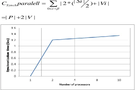
Since an entry of a Synch file Si is two times larger than an entry of the source rank vector Vi.The synchronization cost between processors will be:
i
Synch Vi
Si paralell
C
0
| | ) 2 | | ( * 2 |
| | 2 |
|P V
Figure-9: Synchronization time vs. number of processors
The local CostRank scores have to be synchronized among the ten processors to obtain the final rank to be used in the next iteration step. Figure 9 concludes the synchronization time per number of processors. Each processor needs to receive an updated file from the neighbor host through master (synchronize) machine and processes the update, then sends the updated file to the next neighbor host through master machine. The two master machines need to replicate the data between them. Communication time is incurred when message passing takes place between machines. Synchronization overhead is incurred when the master machine has to wait for synchronization from other machines especially when the number of machines increases, The synchronization overhead maintains about the same percentage (slightly increased due to waiting time) when number of machines increases, whereas the percentage of communication overhead as you see in figure 10 grows with the number of hosts that waits for task completion on the slowest machine. Time devoted in communication and synchronization with other processors was calculated using the following formulas:
Ts pTp
Tq
Ts Cp
[image:4.595.315.542.170.295.2]Tq
[image:4.595.53.282.180.331.2]Figure-10: Communication time vs. number of processors
Figure 11 shows that the standard of residual errors increases when the synchronization interval increases and when the number of processors participating in computation increases as in 2, 4. 8 and 10 processors. The average residual error calculated from synchronizing the local rank scores after every 5 consecutive steps is less than 0.020. This value is acceptable for our research purpose. We thus set the synchronization interval to 5 to be reported in experimental results.
Figure-11: Residual Error
3.5
Execution times
The execution times estimated in this model should by theory, be equivalent to the serial execution time divided by the number of processors, given the assumptions of serialized network transfer between hosts and constant computational time per processor. Let Tpi be the computation time for a CostRank per processor i, Sti is the time to synchronize synch files. The execution time can then be estimated as:
i
ti
Executionparalell Tpi Synch
Time
0
| |
2 | |
[image:4.595.315.544.470.573.2]As the Serial CostRank execution time is divided into β portions, the outline of all portions Tpi will be equal to Ts /β in addition to two synchronized files received from Pβ-1 and Pβ+1(Overhead).
Figure-12: Total Execution times
Our analogous and load balancing scheme indorsed us to load and distribute the matrices to the processors without overloading the memory on any particular machine. Figure 12 presents the execution time of the CostRank algorithm against the number of processors. For the simple distribution (equal number of rows on each processor), the runtime displays oscillations as the number of processors increases. This behavior is smoothened by the load-balancing distribution. Because our algorithms are so sensitive to the communication pattern in the matrix-vectormultiply operation, we believe that these peaks correspond to local maxima in the communication patterns.
3.6
Speedup time
[image:4.595.54.281.581.744.2]is the ratio of the time taken to calculate the rank on a single processor to the time required on a given parallel computer with p processors
Tp Ts S
[image:5.595.315.544.121.276.2]Ts is the time taken on one processor in serial algorithms.Tp is the time taken on p processors.
Figure-13: Speedup vs. number of processors
The parallel simulated CostRank algorithm is shown in figure 13. We plotted the speed up of our parallel simulated algorithm versus the number of processors. In this graph, speedup is defined to be the ratio of time for the serial CostRank algorithm execution to the time for the parallel algorithm execution. Notice that the speedup time is sharply increased when we did the experiments using only 2 hosts: that is due partitioning of the graph file, and the reduction of the speed up time due to the overall loads slump on each processor.The overall increment slightly reduced when we used 4 hosts that is due to the overhead of synchronization process and load balancing.There was gradual increase we got when we used 8 and 10 hosts.
3.7
Cost of parallel algorithms
The cost of a analogous algorithm on a parallel system with p processors, denoted by Cϸ, is defined as the product of the parallel runtime for each processor and the number of processors used. Intuitively, this is the amount of processor-time working together to calculate the cost ranking in parallel:
Tp p* C
Figure 14 presents the computation time of the CostRank algorithm against the number of processors. The computation time displays sharp decline as the number of processors increases. This is due to load distributions on processors working together to calculate the cost ranking in parallel.
Figure-14: Computation time of the CostRank algorithm against the number of processors
3.8
Efficiency of parallel algorithms
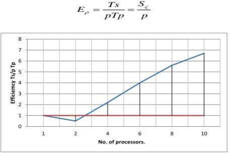
Eϸ is the segment of the parallel runtime that the analogous system is doing effective work. It is given:p S pTp
[image:5.595.53.282.132.261.2]Ts E
Figure-15: Algorithms’ efficiency vs. no. of Processors
Efficiency is defined as speedup divided by the number of processors. Ideal efficiency is always 1, and anything above 1 is super-linear. Values less than 1 indicate withdrawing returns as more processors are added as you can see in figure 15.
3.9
Load Balancing
The load of a parallel program must be balanced among processors to achieve higher utilization of processing resources.To accelerate the CostRank computation we equally distributed the binary graph file among all the processor using following function:
p S Si
[image:5.595.54.284.600.733.2]If „p‟ represents the total number of processors and „S‟ represents the total number of states in the binary graph file then we distributed the states based on the unique state-ID going from 0 to S-1 Every processor is set to handle a particular value in the range of the function i.e. 0 to Si All states having state-ID whose satisfies a particular processor‟s value. To achieve this we needed to implement Greedy algorithm with round robin to distribute the tasks according number of keys in table partition to multiple processors as we see in figure 16. In heterogeneous hardware we cannot determine the exact execution time
Figure-16 Greedy algorithm with round robin
0 1 2 3 4 5 6 7 8
1 2 4 6 8 10
Eff
ic
ie
m
cy
Ts/p
Tp
No. of processors.
P1 P2 P3
T 3
P1 P2 P3
T 1
T 2
T 3
T 4
T 5
T=Task Execution Time
T 2
T 1
T 4
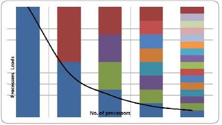
[image:5.595.313.544.620.749.2]22 As we can see in figure 17 due to the states distributions
[image:6.595.53.282.141.270.2]across hosts and processors and due to the use of greedy algorithm with round robin technique shown in figure 16, the load per processor reduces sharply with the number of hosts we used during our experiments.
Figure-17: Processors loads vs. number of processors
Based on our observations, this partitioning scheme yields an agreeable load balancing. This is a result of the uniform distribution of states within the graph file.
4.
CONCLUSIONS
In this paper, we have presented a new parallel algorithm to calculate the CostRank of a network. We have put into practice a developed algorithm to speed up the execution of CostRank computation through the use of graph file partitioning-based techniques. We have untaken the implementations of CostRank in a parallel environment models for one-dimensional sparse matrix partitioning on a modified research page results in a significant reduction in communication overhead and in per-iteration runtime. We implemented conventional load balancing breakdown methods. Our experiments on a gigabit PC cluster have shown that our algorithm models consistently and substantially decreased distributed per-iteration communication overhead, resulting in high reductions of per-iteration run-time when compared to the Serial Cost Rank alternative.We implemented and tested our algorithm on a cluster of ten machines, networked via a Gigabit Ethernet. To study its efficiency, we performed several tests using out-vector files synthesized from the real networked data. The given results are quite encouraging.We have proposed a Partition-based CostRank algorithm that can efficiently run on a parallel environment. We also provided a visible analytical discussion in terms of I/O and synchronization cost, and memory usage, of the algorithms.Our algorithm will run on any number of processors with the optimal cost.
5.
REFERENCES
[1] T.H. Haveliwala. Topic-sensitive pagerank. Proc. of the 11th WWW Conf., 2002
[2] S.D. Kamvar, T.H. Haveliwala, C.D. Manning, and G.H. Golub. Exploiting the block structure of the web for computing pagerank. Preprint, March 2003.
[3] T.H. Haveliwala. Efficient encodings for document ranking vectors. Technical report, Stanford University, November 2002.
[4] U.V. Catalyurek and C. Aykanat. Hypergraph-Partitioning-Based Decomposition for Parallel Sparse-Matrix Vector Multiplication. IEEE Transactions on Parallel and Distributed Systems, 10(7):673–693, 1999. [5] Thaier Hamid and Carsten Maple, IJCA Special Issue on
Network Security and Cryptography Number 1 2011, ISBN: 978-93-80865-66-7.
[6] U.V. Catalyurek and C. Aykanat. A Fine-grain Hypergraph Model for 2D Decomposition. In Proc. 15th IEEE International Parallel and Distributed Processing Symposium, San Francisco, CA, 2001.
[7] G. Karypis, K. Schloegel, and V. Kumar. ParMeTiS: Parallel Graph Partitioning and Sparse Matrix Ordering Library, Version 3.0. University of Minnesota, 2002. [8] B. U¸car and C. Aykanat. Encapsulating multiple
communication cost metrics in artitioning sparse rectangular matrices for parallel matrix–vector multiples. SIAM Journal on Scientific Computing, 25(6):1837– 1859, 2004.
[9] A. Arasu, J. Novak, A. Tomkins, and J. Tomlin. Pagerank computation and the structure of the web: Experiments and algorithms. Proc. of the 11th WWW Conf.,2002. Poster Track.
[10]K. Bharat, B.W. Chang, and M. Henzinger. Who links to whom: Mining linkage between web sites. Proc. of the IEEE Conf. on Data Mining, November 2001.
[11] Aleksandar Trifunovic. Parallel Algorithms for Hyper graph Partitioning. Ph.D. thesis, University of London 2006.
[12]Y. Chen, Q. Gan, and T. Suel. I/O-efficient techniques for computing pagerank. Proc. of the 11th ACM CIKM Conf., 2002.
[13] S. Chien, C. Dwork anf R. Kumar, and D. Sivakumar. Towards exploting link evolution. Workshop on Algorithms and Models for the Web Graph, 2001. [14]Russell Power, Jinyang Li. Piccolo Building fast,
distributed program with partitioned tables.
[15] Arnon Rungsawang and Bundit Manaskasemsak, PageRank Computation Using PC Cluster, Dongarra, D.