Automatic Measurements of the Performance Parameters of Practical Phase Locked Loops

Automatic Measurements of the Performance

Parameters of Practical Phase-Locked Loops

Dina M. El-Laithy

Communications Engineering Department

Modern Academy of Engineering and Technology

Cairo, Egypt

Abdelhalim Zekry

Communications Engineering Department

Faculty of Engineering Ain shams University

Cairo, Egypt

Mohamed Abouelatta

Communications Engineering Department

Faculty of Engineering Ain shams University

Cairo, Egypt

ABSTRACT

An important issue in PLL design and manufacture is to simulate, measure, and verify its performance and key parameters for achieving goals of good time and frequency domain responses, as well as good noise and jitter performance. In this paper, we will introduce our new method that is capable of simulating and measuring automatically the PLL key parameters, such as the hold-in range and the pull-in range. Performance parameters for the PLL, such as loop gain, damping factor, natural frequency and settling time, can be simulated and measured concurrently. This method will help to shorten the time of measurements. This work presents an automatic testing method for the PLL using circuit simulator and practical circuit implementation. An industrial CMOS PLL is used to implement the PLL. Good agreement between the simulation and experimental is results is found.

General Terms

Electronic design, Communications, Simulation, Hardware

Keywords

Phase locked loop, tracking range, capture range, natural frequency, damping factor

1.

INTRODUCTION

Phase-Locked Loop (PLL) has received a wide range of applications in modern data-communications, telecommunications, wireless communications, as well as computer related microprocessor, data bus, video and audio ICs [1]. There has been increasing demand for high speed and low noise data receivers such as disk drive read/write channels, and high speed modems, etc. In such applications, clock recovery is required to show better performance for the extraction of timing from incoming data [1]–[4]. Of various techniques, such as the tank circuit, the surface acoustic wave (SAW) filter, the crystal filter, and the PLL, the PLL is one of the most desirable components for timing extraction because of its low cost, high integration, and easy and wide availability [5],[8]. An important problem in PLL design and manufacture is to simulate, measure, and verify its loop response and key parameters in order to achieve goals of good time and frequency domain responses, as well as good noise and jitter performance [5]. The capture range, the tracking range and the settling time are commonly used to describe the dynamic behavior of the PLL. The settling time is a very important parameter, especially in wireless communication. There are several methods to improve the settling time [6].

This paper is organized as follows. Section 2 presents the

the PLL. The simulation results are discussed in Section 3. Section 4 illustrates the experimental results. The conclusions are given in Section 5.

2.

ANALYZING THE CLOSED LOOP

PERFORMANCE PARAMETERS OF

THE PLL

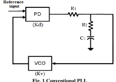
The PLL is shown in Fig. 1. It is composed of a digital phase detector which is an XOR, a loop filter and a voltage-controlled oscillator. The first-order loop filter is composed of the resistors R1 and R2 and the capacitors C1. Its transfer

function F(s) is given by [7],[9]:

2

1 2 1 ( )

1 ( )

s F s s



 

  (1)

Where τ1 = R1C1 and τ2 = R2C1. For this filter, the PLL closed

loop transfer-phase function becomes [7],[9]:

which are used as the characterizing parameters of PLL and are given by [7]:

= and = (3)

VCO. The term Kd Ko is called the loop gain KL and has the

dimension of angular frequency (rad S-1).

KL = Kd Ko (4)

The performance of the PLL depends on the individual components and system transfer function. For a damping factor = 0.7, 3db becomes equal 2.05 n.

The loop-filter component values used in this work are R1=12

KΩ, R2=0.5 KΩ and C1=10 nF. We set the center frequency fo=

84 KHz and Ko =2π*16.88 Krad/Sec.V. The phase detector

used is the XOR-PD which has Kd=Vdd/π = 1.6 rad/V for

supply voltage Vdd = 5 V. As per Eq. 3, the natural frequency

n = 36.8 Krad/sec and the damping factor is equal to 0.092.

All these values are listed in Table 1.

To complete the performance analysis of the PLL, the hold-in range and the pull-in range must be determined for specifying the frequency range in which the PLL can be operated. The pull-in range ∆ P is equally often called the capture range of

the PLL, and it is the frequency range over which the PLL can acquire lock. Accordingly, the hold-in range ∆ H is called the

tracking range of the PLL, and it is the frequency range over which the PLL can maintain lock. Usually the tracking range is greater than or equal to the capture range. They are given by [4]:

= π , = (5)

For this work and assuming practical phase locked loop operation, we set the center frequency fo = 13KHz and the

VCO gain Ko =2π*5.2 Krad/Sec.V. The XOR-PD gain Kd =

1.6 rad/V. Set the damping factor = 0.7 and the natural frequency n = 6.5 Krad/sec, the loop-filter components should

be R1=10 KΩ, R2=2.3 KΩ and C1=100 nF.

As per Eq. 5, the capture range ∆ P = 35.3 Krad/sec and the

tracking range ∆ H = 81.5 Krad/sec. which leads to ∆fcapture =

5.6 KHz and ∆ftracking = 13 KHz. All these values are listed in

Table 2.

To measure the natural frequency n and damping factor of

the PLL, we apply a disturbance to the PLL which forces the system to settle at a different stable state. This is done by modulating the reference frequency with a square-wave. The corresponding test circuit is shown in Fig. 2. The settling time Ts is usually practically defined to be the time when the output frequency approaches the input reference frequency within a predefined margin [6], and can be measured by using the same test circuit.

Fig. 2 A block diagram for the measurement of natural frequency ωn , damping factor ζ and settling time Ts

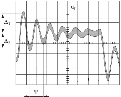
The modulating frequency must be chosen to be much smaller than the center frequency-for example, 1 KHz. If the frequency of the signal generator is abruptly changed, the output signal uf of the loop filter performs a damped

oscillation on every transient of the 1 KHz of the square wave and settles at a stable level thereafter. The natural frequency

n and the damping factor can be calculated from the

waveform of uf shown in Fig 3.

The damping factor can be calculated from the ratio of the amplitudes of two subsequent half-waves A1 and A2. The

damping factor is given by [7]:

π (6)

The natural frequency n is calculated from the period T of

one oscillation in Fig. 3 according to [7]

n =

(7)

And the settling time Ts is the time required for the PLL to settle to a new frequency [7], and can be calculated directly from the figure.

To measure the capture range (∆ P) and the tracking range

(∆ H) of the PLL, we use the same test circuit of Fig. 2 with

changing the square wave generator to a triangular wave generator.

To make capture and tracking range measurements, the PLL must be forced in and out of lock. This can be accomplished by sweeping the reference frequency automatically by using the FM modulator. The period of the sweep is 10 ms. It is very important to use a sweep time that is slow enough to eliminate capture transient effects.

Fig. 4 shows the output signal uf of the loop filter during the

automatic sweeping. The capture and tracking range can be calculated from the waveform of uf as shown in the figure.

Fig. 4 The Loop-filter output uf shows the capture and tracking range of the PLL.

Starting from the left of Fig. 4, we can see that the PLL is not following the input signal; some instances it goes to out of lock. As the sweeping voltage increases the reference frequency increases, the PLL acquires lock and starts to track the changing input frequency. Where the PLL acquires lock is called the lower capture frequency. As the frequency increases further, the PLL tracks, and then finally loses lock. Where the PLL loses lock is the upper frequency of the tracking range. The input frequency will finally start to decrease and the PLL will lock again, this point represents the upper frequency of the capture range. As the input frequency continues to decrease, the PLL tracks, and then finally loses lock. Where it loses lock again represents the lower limit of the tracking range. Now we can determine the tracking and the capture range as follow:

The tracking range ( ) = Upper tracking frequency – Lower tracking frequency (8)

The capture range ( ) = Upper capture frequency – Lower capture frequency (9)

3.

SIMULATION RESULTS

Fig. 5 shows the SPICE circuit used to measure the damping factor , the natural frequency n and the settling time Ts. Fig.

6 shows simulated transient responses for the PLL. From Fig. 6, A1 = 0.31, A2 = 0.23, T = 170 us and the settling time Ts =

750 us. Using Eq. 6 and Eq. 7 give = 0.095 and n = 37.1

Fig. 5 Schematic of the PLL to determine the performance parameters by SPICE simulation .

Table 1 Performance summary of the PLL for 1st measurements

Supply voltage 5V

Frequency step 20 KHz

VCO center frequency 84 KHz

VCO's frequency range 17-150 KHz with Ko = 16.88 KHz/V

R1 in loop filter 12 KΩ

R2 in loop filter 0.5 KΩ

C1 in loop filter 10 nF

Natural frequency n

36.8 Krad/sec (calculated)

37.1 Krad/secs (simulated)

31.53 Krad/sec (measured)

Damping factor

0.092 (calculated)

0.095 (simulated)

0.091 (measured)

Settling time Ts

750 us (simulated)

800 us (measured)

To determine the capture and tracking range of the PLL using simulation, Fig. 7 shows the SPICE circuit used. Fig. 8 shows simulated transient responses for the PLL. Performance summaries of this work are also listed in Table 2.

Table 2 Performance summary of the PLL for 2nd measurements

Supply voltage 5V

Input sweep frequency 100 Hz

VCO center frequency 13 KHz

VCO frequency range 5-21 KHz with Ko = 5.2 KHz/V

R1 in loop filter 10 KΩ

R2 in loop filter 2.3 KΩ

C1 in loop filter 100 nF

Natural frequency n 6.5 Krad/sec

Damping factor 0.75

Capture range ∆fP

5.6 KHz (calculated)

5.2 KHz (simulated)

5.2 KHz (measured)

Tracking range ∆fH

13 KHz (calculated)

13.3 KHz (simulated)

13.3 KHz (measured)

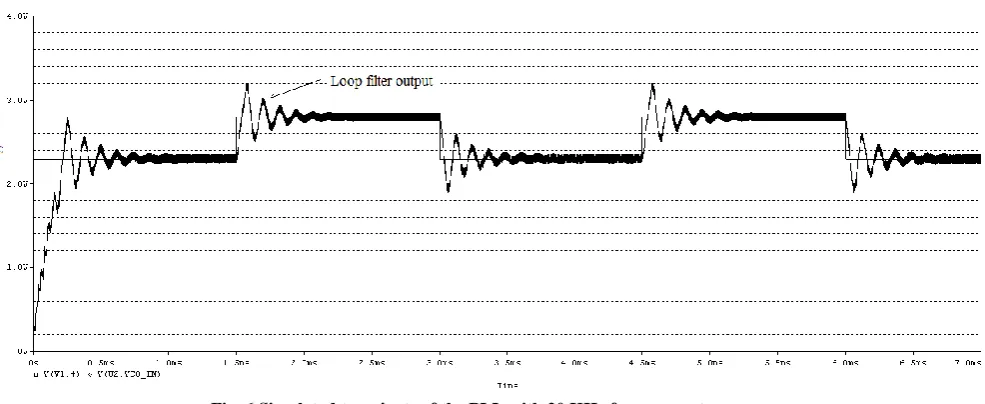
Fig. 8 Simulated transient of the PLL with 100 Hz sweep frequency.

Starting from the left of Fig. 8 leaving the first transient cycle, we can see that the PLL is not following the input signal, sometimes it is out of lock. As the sweeping voltage increases the reference frequency increases, the PLL acquires lock at uf = 2V

and it corresponds to fout = 10.4 KHz and starts to track the

changing input frequency. Where the PLL acquires lock is called the lower capture frequency. As the frequency increases further, the PLL tracks, and then finally loses lock, at uf = 3.8 V which

corresponds to fout = 19.5 KHz. Where the PLL loses lock is the

upper frequency of the tracking range. The input frequency will finally start to decrease and the PLL will lock again, at uf = 3 V

which corresponds to fout = 15.6 KHz. This point represents the

upper frequency of the capture range. As the input frequency contains to decrease, the PLL tracks, and then finally loses lock, at uf = 1.2 V which corresponds to fout = 6.2 KHz. Where it loses

lock again represents the lower limit of the tracking range. Now we can determine the tracking and the capture range from Eq. 8 and Eq. 9:

The tracking range ( ) = 19.5K – 6.2K = 13.3KHz

The capture range ( ) = 15.6K – 10.4K = 5.2KHz

4.

EXPERIMENTAL RESULTS

The practical implementation for the PLL is carried out to verify the results obtained by analytical formulas and computer simulations. The circuits shown in Fig. 5 and Fig. 7 had been completely built and tested in the laboratory and the time response of the PLL was measured

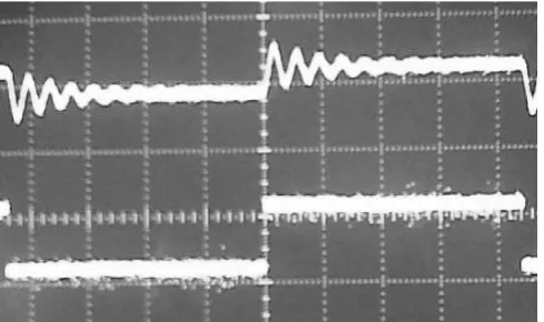
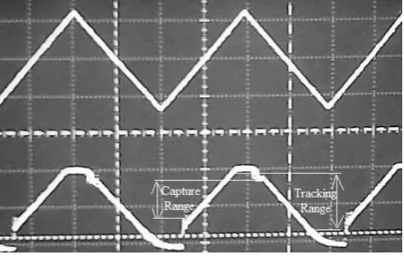
Fig. 9 and Fig. 10, show typical oscillograms of the PLL for measuring the performance parameters and measuring the capture and tracking range respectively. The measured natural frequency n = 31.53 rad/sec, the damping factor = 0.091, the

settling time Ts = 800 us. The measured capture range ∆fP = 5.2

KHz and the measured tracking range ∆fH = 13.3 KHz. Results of

this experimental work are also listed in Table 1 and Table 2.

It is clear from the results in these tables that the calculated, the simulated and the measured PLL performance parameters agree with each other within the practical component tolerances and the measurement errors as well as the model approximations in SPICE. Indeed, The agreement is satisfactory.

Fig. 10 Measured transient of the PLL with 100 Hz sweep frequency.

5.

CONCLUSION

In this paper, a complete study to determine the performance parameters of PLL is achieved. Fast and direct analysis to measure PLL capture and tracking range is presented. A 100 Hz sweep triangular signal is used for monitoring the output frequency while the PLL is forced to go in and out of lock. A quick and simple view of the PLL's capture and tracking range are displayed in one direct measurement which helps to shorten the time of measurements. We proved also that both the calculated and simulated PLL parameters are in close agreement with the measurement results. Therefore one can use them to design the PLL and expect no appreciable deviation from practical behavior.

6.

ACKNOWLEDGEMENT

The authors would like to thank the Department of Electronics & Communication Engineering, Ain Shams University, for providing its laboratory and library facilities.

7. REFERENCES

[1]Mike LE, “A new method for simultaneously measuring and analyzing PLL transfer function and noise processes,” Ph.D. dissertation, Univ. California, Berkeley, June 2002. 1111

[2]Mozhgan Mansuri, Dean Liu, and Chih-Kong Ken Yang et al., “Fast frequency acquisition phase-frequency detectors for Gsamples/s phase-locked loops,” IEEE Journal of Solid-State Circuits, Vol. 37, No. 10, Oct. 2002, pp. 1331–1334.

[3]W. C. Lindsey and C. M. Chie, Phase-Locked Loops. New York. IEEE Press, 1986.

[4]C.S. Vaucher. "An adaptive PLL tuning system architecture combining high spectral purity and fast settling time," IEEE Journal of Solid-State Circuits, Vol. 35, pp. 490-502, 2002.

[5]J Floyd M. Gardner, Phaselock Techniques. John Wiley &Sons, 1979.

[6]Texas Instruments, “Fractional/integer-N PLL basics”, SWRA029, edited by Curtis Barrett, wireless communication business unit, 1999

[7]R. E. Best, Phase-Locked Loops: Theory, Design and Applications. New York, NY: fifth edition, McGraw-Hill, 2003.

[8]William F. Egant “Phase-Lock Basics”. Second Edition. Copyright 2008 by John Wiley & Sons, Inc.

[9]Paul Brennan, “Phase-Locked Loop notes”, E771 Electronic Circuits III, University College London, 2000.