Consumption of private goods as substitutes for environmental goods in an economic growth model

Consumption of private goods as

substitutes for environmental goods in an

economic growth model

Antoci, Angelo and Galeotti, Marcello and Russu, Paolo

University of Sassari, University of Florence

2005

Consumption of Private Goods as Substitutes for

Environmental Goods in an Economic Growth Model

A. Antoci1_{, M. Galeotti}2_{, P. Russu}1

1

DEIR, University of Sassari via Sardegna 58, 07100 Sassari, Italy

antoci@uniss.it 2

DiMaD, University of Florence

Received: 21.07.2004 Accepted: 04.02.2005

Abstract. We analyze growth dynamics in an economy where a private good can be consumed as a substitute for a free access environmental good. In this context we show that environmental deterioration may be an engine of economic growth. To protect themselves against environmental deterioration, economic agents are forced to increase their labour supply to increase the production and consumption of the private good. This, in turn, further depletes the environmental good, leading economic agents to further increase their labour supply and private consumption and so on. This substitution process may give rise to self-enforcing growth dynamics characterized by a lack of correlation between capital accumulation and private consumption levels, on one side, and economic agents’ welfare, on the other.

Furthermore, we show that agents’ self-protection consumption choices can generate indeterminacy; that is, they can give rise to the existence of a continuum of (Nash) equilibrium orbits leading to the same attracting fixed point or periodic orbit.

Keywords: self-protection choices, indeterminacy, undesirable economic growth.

1 Introduction

pollution generated by industrial activities or urban traffic (for example, double-glazing) and drugs to treat respiratory illnesses caused by air pollution. Certain consumption expenditures on the part of city dwellers are conditioned, at least in part, by defensive reasoning. Consider the choice of using a car as a means of transport, a choice which may be caused by air pollution: individuals who would have preferred to go by bicycle are forced to use their car because the air is unbreathable. The shortage of parks and areas where children can play without the constant supervision of adults imposes further consumption expenditures. The massive use of home entertainment by children is partly a result of the lack of such areas, of the degradation of the urban environment and of the need to protect children from the dangers of urban traffic. The shortage of green space can induce individuals to purchase an entrance ticket for a protected nature area or to spend money on a day out to find a place to enjoy nature and leisure activities. Another possible expenditure could be joining a gym, substituting physical activity in a park in the open air with exercise carried out in a sports centre.

However, these are only “textbook” examples; the literature of environmental economics suggests that the category of defensive environmental spending can be interpreted in a very broad manner, comprising a vast range of consumptions that derive in part from environmental degradation, but are not merely a response to it. The literature on this argument (see, e.g., [1–8]) supports the idea that individuals may react to environmental deterioration in a great variety of ways. When the environment deteriorates, individuals are more incentivated to adopt consumption patterns based on the use of private goods rather than on the use of free access environmental goods: spending a day on an uncontaminated beach close to home can be more rewarding (and generally requires the consumption of a lesser quantity of private goods) than spending a day in town; nevertheless, the latter option becomes relatively more remunerative if the quality of the beach is compromised.

as a substitute for the environmental good and can be saved and accumulated as capital. The environmental good is deteriorated by the pollution caused by the average consumption activity of the private good in the economy.

At every instant of time each economic agent has to choose the allocation of his endowment of time between leisure and the production process of the private good and the allocation of the output between present consumption and accumulation of capital. Since the negative impact on the environmental good of each agent’s consumption choice is negligible (agents being a continuum), he doesn’t take this into account in his consumption choices.

In this context, by working harder, economic agents can consume more in the present and/or in the future (via accumulation of capital) and consequently can benefit from a better self-protection against environmental deterioration in the present and/or in the future. Thus, economic agents may react to the deterio-ration of the environmental good by increasing the production and consumption of private goods; by doing so, they cause a further depletion of the environmental resources, which can, in turn, force agents to further increase private consumption and accumulation.

The paper is organized as follows. Section 2 illustrates the main results of the paper, comparing them with those of related literature. Section 3 defines the model. Sections 4–9 analyze the dynamics. Section 10 outlines the conclusions.

2 Related literature

The mechanism of economic growth that we intend to analyze is based on the hypothesis that the consumption of the private good by each economic agent contributes to the depletion of the environmental good, and therefore generates a negative externality (in the model the agents do not take into consideration the negative impact of their choices on the environmental good) on the other agents. Consequently, in our model, defensive consumption choices may be classified as self-protective choices “transferring” the negative externalities to other individu-als [9]; that is, each victim of negative environmental externalities defends himself by implementing the defensive consumption which generates further negative externalities for other individuals.

[10], who demonstrated that, in a context where individuals do not cooperate (i.e., they do not “internalize” the externalities), the outcome is a degree of self-protection that exceeds the socially optimal level. It implies that, if the individuals protect themselves by consuming private goods, the expected outcome is an excess in the consumption of private goods.

Such analysis has been extended to a dynamic context in several works1; Antoci and Bartolini [1,2,12], have studied the dynamics of labor supply under the assumption of bounded rationality (i.e., agents don’t have perfect foresight about the future evolution of state variables), neglecting the accumulation of capital; in particular, they have analyzed evolutionary games where individuals have to choose their labor efforts from among a finite number of options and where the better performing choices become widespread in the population of individuals at the expense of those that are less rewarding. The analysis of these models shows that economic dynamics can present two or more locally attracting fixed points characterized by an inverse correlation between labor effort (and private consumption level) and individuals’ welfare.

Bartolini and Bonatti [3] assume perfect foresight and analyze a model with-out capital accumulation where economic agents choose their (identical) labor ef-forts from among a continuum of values. In this context, they obtain results which are analogous to those obtained in the above-mentioned evolutionary games, show-ing that such results do not depend on the bounded rationality assumption.

Bartolini and Bonatti [4] analyze a discrete time perfect foresight dynamic with capital accumulation; however, their model shows a single fixed point which is a saddle point. Their analysis limits itself to the sensitivity analysis of the fixed point with respect to the variations of the parameters of the model.

The present work intends to contribute to this line of research by showing that, even in a model of capital accumulation and perfect foresight, there may exist multiplicity of fixed points and that there may be no correlation between private consumption and capital accumulation levels in such states and the welfare of the economic agents; fixed points with high consumption and accumulation levels

1_{All this works build on the well known work of Hirsch [11] who suggests that individuals’}

can be Pareto-dominated by others characterized by lower levels. Furthermore the substitution process between environmental and produced goods may have effects on the stability of fixed points and may generate closed orbits; self-protection choices can produce indeterminacy, that is the existence of an infinite number of equilibrium orbits leading to the same (locally) attractive fixed point or periodic orbit. When indeterminacy occurs, given the initial values of the capital stock and the environmental good, the economy can reach the attracting fixed point (or the periodic orbit) by following an infinite number (a continuum) of growth paths, each characterized by different consumption patterns and welfare levels. Consequently, the economy may experience very different welfare situations2. Starting from different initial values of the state variables, it can reach different fixed points (characterized by different welfare levels). Furthermore, when in-determinacy occurs, each fixed point (or periodic orbit) can be reached along an infinite number of possible orbits, each of them giving rise to possibly different welfare levels3.

Finally, there is a strand of literature (see, e.g., [15–19]) that highlights other mechanisms according to which natural resources abundance may inhibit eco-nomic growth (for a review of this literature see [20]). However, according to the mechanisms analyzed in the above-mentioned literature, economic growth always generates welfare improvements.

3 The model

There exists a large number (a continuum) of identical economic agents. Since all agents are identical, we can consider the choice process of a representative agent. We assume that, at each instant of timet, representative agent’s welfare depends on three goods:

1. Leisure1₋l(t), wherel(t)is representative agent’s labor input.

2. A free access (renewable) environmental goodE(t). 2

For a review of macroeconomic models featuring indeterminacy see [13]. 3

3. A private good which can be consumed either as a substitute for the environ-mental good c₂(t), i.e., as a self-protection device against environmental deterioration, or in order to satisfy needs different from those satisfied by the environmental resource c1(t).

We assume that the representative agent’s decision problem is

max

c1,c2,l

∞

Z

0

lnc1+aln(E+bc2) +dln(1−l)e−rtdt, (1)

˙

k=lαk1−α_Ω

−c₁₋c₂, (2)

˙

E =βE( ¯E₋E)₋γ(¯c1+ ¯c2)E, (3)

wherea,b,d,r,α,β, γ andE¯ are strictly positive parameters, k(t)represents physical capital accumulated by the representative agent andl(t) is the represen-tative agent’s labor input;k˙andE˙ denote the time derivatives ofkandE.

The representative agent has to choose the functions c1(t), c2(t) and l(t)

to maximize the integral in (1). Note that, according to the (instantaneous) utility functionlnc1+aln(E+bc2)+dln(1−l), an increase of substitutive consumption c2(t)compensates the negative effect deriving from a reduction ofE(t).

Equation (3) describes the dynamics ofE(t); note that the value of the pa-rameterE¯ can be interpreted as the endowment of the environmental good in the economy, i.e., the state variableEwould reach such a value without the negative effect due to the average economy-wide consumption¯c1 + ¯c2. The assumption

At each instant of time, the representative agent produces the quantity of output lα_k1−α_{Ω and, according to the equation (2), the difference between the}

productionlαk1−α_{Ωand the consumption c}

1+c2 is accumulated as productive

capital.

In the production functionlαk1−α_{Ω,Ωrepresents a positive externality due}

to the economy-wide production activity. We assume that α < 1; so, with Ω

constant, the production function exhibits a constant return-to-scale technology (i.e., it is a homogeneous function of degree 1). In accordance with the literature on economic growth with externalities (see, e.g., [13, 21]), we model the positive externality as follows

Ω := ¯lδk¯ε,

where δ and ε are strictly positive parameters and ¯l(t) and ¯k(t) represent the average use of labor and capital in the economy, respectively. When the average capital or labor input goes up, the productivity oflandkgrows in thatΩis increa-sing in¯land in¯k. We assume that average values are considered as exogenously given by the representative agent when optimizing. This assumption is plausible in a context in which there is a very large number of agents (in particular, we have assumed that they are a continuum); so, each agent considers as negligible the impact that his own choices may have on the average values of economic variables. A consequence of this assumption is that the growth dynamics we shall analyze are not optimal; however, each growth path followed by the economy represents a Nash equilibrium; that is, no agent has an incentive to modify his choices if the choices of the others are fixed.

Since all agents are identical, they make the same choices; consequently, the average values¯c1(t),¯c2(t),l¯(t),¯k(t)coincide (ex post) with the values ofc1(t), c2(t), l(t), k(t) chosen by the representative agent. Note that, by substituting

¯

l(t) = l(t) and ¯k(t) = k(t) in the production function lα_k1−α_{Ω, we obtain}

the functionlα+δk1−α+ε_{, i.e., the function that would be considered by a social}

For space constraints, we restrict our analysis here to the study of caseε < α; this assumption rules out the possibility of unbounded growth ofk; the caseε_≥α

will be considered in a future study.

The Hamiltonian function for our problem is

H(E, k, λ, θ, l, c1, c2) = lnc1+aln(E+bc2) +dln(1−l)

+λ(lαk1−α_Ω

−c₁₋c₂)

+θ βE( ¯E₋E)₋γ(¯c1+ ¯c2)E,

whereλ andθ are the co-state variables associated withkandE respectively. By applying the maximum principle we obtain that the dynamics ofc1(t),c2(t), l(t),k(t),E(t) must satisfy the following conditions

∂H ∂l =−

d

1₋l+αλl

α−1_k1−α_{Ω = 0, (4)}

∂H ∂c1

= 1

c1 −

λ= 0, (5)

∂H ∂c2

= ab

E+bc2 −

λ_≤0, c_{2 ≥}0, c₂∂H ∂c2

= 0, (6)

˙

k= ∂H

∂λ =l

α_k1−α_Ω

−c1−c2, (7)

˙

λ=rλ₋∂H

∂k =λ r−(1−α)l

α_k−α_{Ω, (8)}

˙

E = ∂H

∂θ =βE( ¯E−E)−γ(¯c1+ ¯c2)E, (9)

where¯c₁,c¯₂,¯l,¯kmust be replaced byc₁,c₂,l,kin expressions (4)–(9) and the control variablesc1,c2,lare determined by conditions (4)–(6). Notice that, in our

model the control variablesc1 andlare always strictly positive andl <1.

We omit the dynamics of the co-state variableθ since equations (7)–(9) do not depend on it (precisely because ¯c1 andc¯2 are considered exogenous by the

representative agent). Furthermore, we assume the usual transversality condition

lim

t→∞k(t)λ(t)e

−rt_{= 0,}

4 Dynamics withc₂ = 0

From (6) it follows that, if the condition

ab

E −λ≤0 (10)

is met, then the representative agent choosesc2 = 0; i.e., he doesn’t consume the

private good as a substitute for the environmental good. Otherwise, he chooses

c2 >0. Condition (10) is satisfied if, givenλ, the value ofEis high enough. The

dynamics withc2 = 0are analyzed in [22], where the possibility of substitution

between the private good and the environmental good is not considered. In this section, the basic analytical results of the said paper are illustrated.

Whenc2 = 0, system (7)–(9) is decoupled in the planar system given by (7)

and (8) and the non-autonomous differential equation (9). We can easily observe that at most one fixed point, sayS′_{, exists, with the following coordinates}

k′

=

1₋α r

_α

α+d

α+δ

1

α−ε

,

λ′

= 1−α

rk′ ,

E′

= ¯E₋ γr β(1₋α)k

′

.

Such a fixed point exists only if (10) is satisfied, which requires, coeteris paribus, the endowment of the environmental good, E¯, to be sufficiently high and the negative impact, γ, of average consumption on the environmental good to be sufficiently low.

The stability of the fixed point is described by

Theorem 1. Let

p:= α−ε

d(1₋α₋δ) +α, q := (1−α)

d(1₋α₋δ) +α+ (α+d)ε d(1₋α₋δ) +α .

Then:

(i) If p >0,S′

(ii) If p <0 and q >0,S′

is a saddle with a one-dimensional stable manifold.

(iii) If p <0 and q <0,S′ _{is a sink.}

If case (i) holds, given the initial values of k and E, there exists (at least locally) a single initial value ofλ(determined by the representative agent) from which the economy approaches the fixed point.

Note that condition (i) is satisfied if α +δ _≤ 1, where α and δ are the exponents ofland¯l, respectively, in the production function.

The fixed point cannot be (generically) reached if (ii) holds.

Vice versa, when (iii) is satisfied, given the initial values ofkandE,there exists a continuum of initial values ofλleading to the fixed point. In other words there exist an infinite number of (Nash) equilibrium orbits that the economy may follow to reach the fixed point. Along each orbit no economic agent has an incentive to change his choices, given other agents’ choices.

Observe that the parameters r (discount rate), E¯ (endowment of the envi-ronmental good),γ (impact of average consumption on the environmental good) play a role in the existence of the fixed point (condition (10)), but don’t affect its stability properties.

Theorem 2. Whenδcrosses the value

¯

δ:= 1₋α+α

d +

(α+d) 1₋α

an attracting limit cycle (through a Hopf supercritical bifurcation) arises for

δ >δ¯.

Proof. Proofs of the above theorems are given in [22].

When an attracting orbit exists, by following such an orbit the economy may enter the region of the plane(λ, E)wherec2 >0. However, this is not the case

if the periodic orbit is small enough. Antoci, Brugnano and Galeotti [22] show, through numerical simulations, that the periodic orbit expands as the bifurcation parameterδincreases.

5 Fixed points in the regimec₂ >0

It is easy to check that, in the regimec₂ >0,there always exists a fixed point at which the environmental good is completely depleted, that isSe = (k, c1, E) =

(ek,_ec1,0),c1 = 1_λ with

e

k=

r

1₋α

α(1 +a) +d α(1 +a)

1

ε−α

, _ec1 =

α(ek)1−α+ε

α(1 +a) +d.

Denote by S = (k∗_{, c}∗

1, E∗) a fixed point satisfying the conditionsE > 0 and c2 >0. ThenE∗, k∗, c∗1 >0andbc∗2 =abc∗1−E∗>0[see (6)].

Theorem 3. S = (k∗_{, c}∗

1, E∗)is a fixed point satisfying the conditionsE >0and c2 >0, if and only if

¯

E =ψ(k∗

) :=m(k∗

)αε++δδ −nk∗, ₍₁₁₎

where

m:= αb(a+ 1)

d

_r

1₋α

α+δ₋1

α+δ

, n:= br(1 +a)

d(1₋α)

α+ d(bβ−γ)

bβ(a+ 1)

,

and, furtherly,k∗

∈ (k₁, k₂),k₁andk₂ being determined by the intersections of the curveE¯ =ψ(k∗_{) with the lines}

¯

E =m1k∗ :=

(abβ+γ)r

(1₋α)β k

∗

, E¯=m2k∗ := γr

(1₋α)βk

∗

.

Proof. See Appendix A.

Remark. S is unique whenever ψ′

(k∗

) does not change sign in (k1, k2) (see

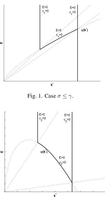
Figs. 1, 2). So, from (11), it follows that there exists at most one fixed point S

ifn _≤ 0 (implyingψ′_(k∗_{) > 0}

fork∗ _{> 0}

), whereas two fixed points (withc∗

2, E∗ _>

0) can exist ifψ(k∗

)has a maximum in (k₁, k₂) (seeFig. 3). Straightfor-ward computations yield that the latter case holds, if and only if

γ < σ < abβ+γ, (12)

where

σ :=

α(a+ 1)bβ+ (bβ₋γ)d(α₋ε)

k*

E

c

2=0

E>0 E=0

c

2>0

E>0 c

2>0

|

ψ(k*)

Fig. 1. Caseσ≤γ.

k*

E

c

2=0

E>0 E=0 c₂>0

E>0 c₂>0

| ψ(k*)

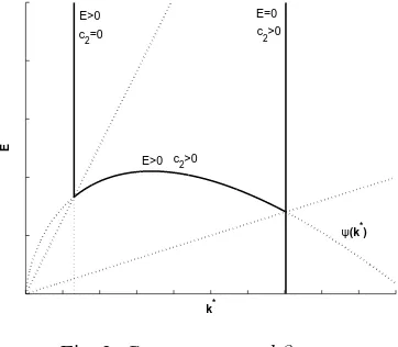
Fig. 2. Caseσ_≥abβ+γ.

Then, if (12) is verified, an interval( ¯El,E¯u)is given, with

¯

El := max

ψ∗

(k1), ψ∗(k2),

¯

Eu :=ψ(k0), where ψ′(k0) = 0, k1 < k0 < k2,

such that for anyE¯_∈( ¯El,E¯u)there exist two fixed points with a strictly positive

Ein the regimec2 >0.

Observe that condition (12) is never satisfied if coeteris paribus, the negative impactγ, on the environmental good of average consumption is high enough.

given the endowment of the environmental good), the intersections between the horizontal straight line passing through it and the continuous lines drawn in each figure give the number of existing fixed points and the corresponding values of

k∗

.

k*

E

E>0

c

2=0

E=0 c

2>0

c

2>0

E>0 |

ψ(k*)

Fig. 3. Caseγ < σ < abβ+γ.

Note that, in Figs. 1–3, the fixed point with the lowest level of capital accu-mulation is the one withE > 0andc2 = 0(when existing). Such a fixed point

would be unique if the private good could not be consumed as a substitute for the environmental good.

Fig. 1 illustrates the caseσ _≤ γ (that is, the case where the negative impact on the environmental good of average consumption is sufficiently high). In such a case at most three fixed points can exist. If the endowmentE¯of the environmental good is high enough, then there exist two fixed points: the one withE = 0and

c2 > 0 and the one withE > 0 andc2 = 0. AsE¯ decreases, then three fixed

points appear: those withE = 0, c2 > 0andE > 0, c2 = 0and a fixed point

whereE > 0andc2 > 0. Finally, ifE¯ is sufficiently low, then only the fixed

point withE = 0exists.

Fig. 2 can be interpreted in a similar way. Unlike in Fig. 1, at most two fixed points can coexist.

Fig. 3 shows the more interesting case, where the highest number of fixed points can exist, i.e., one withE >0andc₂ = 0, two with E >0andc₂ >0, one withE = 0andc2 >0. Such a regime exists if, coeteris paribus,E¯ andγ

6 Stability analysis

6.1 Stability of the fixed point withE = 0

It is easy to check that atSe= (ek,ec1,0)theE-axis is an eigenspace of the Jacobian

matrix, whose associated eigenvalue has the sign ofE¯₋ψ(ek).

The stability ofSeas well as the dynamics in the invariantE = 0plane can be reconducted to the projection on the (k, λ) plane of the c2 = 0 regime, by

replacingdwithd′

:= _a+1d andλwithλ′

:= _a+1λ . Thus, in particular:

Case 1. If δ <1₋α+_dα′, Se is a saddle in the invariant planeE= 0.

Case 2. If δ >1₋α+ α d′ +

(α+d′_)ε

(1−α)d′, Se is a source in the invariant planeE = 0.

Case 3. If 1₋α+_dα′ < δ < 1−α+

α d′ +

(α+d′_)ε

(1−α)d′, Se is a sink in the invariant

planeE= 0.

Therefore, starting from a strictly positive value of E, the fixed point can be (generically) reached by suitably choosingλifE¯₋ψ(ek) <0is satisfied and Case 1 or Case 3 holds. In particular, when Case 3 holds, there exists a continuum of orbits approaching the fixed point, i.e., indeterminacy occurs.

6.2 Stability of the fixed points withE >0_{in the regime}c₂ >0

Straightforward calculations enable the definition of the Jacobian matrixJ(S)

J(S) =

  

A B₋(a+ 1) 1_b

c∗

1

k∗ (1−α)A−r

c∗

1

k∗(1−α)B 0

0 ₋γ(a+ 1)E∗ γ−bβ

b E

∗

  

whereA,B, anddet J(S)are computed in Appendix B. We can distinguish the following subcases.

6.2.1 Caseα+δ _≤1

Theorem 4. If α+δ _≤ 1 andψ′_(k∗₎

6

= 0, J(S) has at least one eigenvalue with positive real part. In particular, if ψ′

(k∗

one-dimensional stable manifold; ifψ′_(k∗_{) < 0}

, S is either a saddle with a bi-dimensional stable manifold or a repellor. In the last case, whenk∗

approaches

k2, a Hopf bifurcation, generically, takes place:S is transformed from a repellor

into a saddle with a bi-dimensional stable manifold.

Proof. See Appendices C and D.

Remember that, in the production function of the representative agent,α is the exponent of labor inputlandδ is the exponent of average labor input¯l. The above theorem says that, ifα+δ_≤1, then the fixed points in the regimeE >0

andc2>0cannot be attractive: that is, indeterminacy cannot occur.

Furthermore, if a fixed point satisfiesψ′_(k∗_{) >0, then it cannot be reached}

(generically) by the economy. If instead the condition ψ′

(k∗

) < 0 holds, then the fixed point has a bi-dimensional stable manifold (and can be reached by the economy) if k∗ _{is near enough to k}

2; otherwise, it may be a repellor. In the

latter case, such a fixed point might be “surrounded”, via a Hopf bifurcation, by a periodic orbit with a bi-dimensional stable manifold.

Remember that, ifα+δ _≤1, the fixed pointS′

in thec2 = 0regime (when

existing) is always a saddle with a bi-dimensional stable manifold. Ifα+δ _≤1

and σ _≤ γ (see Fig. 1), the fixed point satisfying E > 0 and c2 > 0 cannot

be (generically) reached by the economy, being a saddle with a one-dimensional stable manifold. The fixed point withE = 0cannot be reached (starting from a strictly positive value ofE) ifE¯is high enough, that is, whenE > ψ¯ (k∗₎

and the Jacobian matrix has a strictly positive eigenvalue in theE-axis direction.

Observe that both the fixed point withE= 0 and the one withc2= 0 can be

saddles with bi-dimensional stable manifolds. In such a case a bi-stable dynamic regime occurs: the economy can approach either fixed point depending on the initial values ofEandk.

Analogous observations can be made about Figs. 2 and 3.

6.2.2 Caseα+δ >1

Theorem 5. Wheneverα +δ > 1, an attractor can exist, with E > 0, in the

Proof. Applying formulae (C.2)–(C.5), it is easy to see that the fixed pointS is an asymptotic attractor, if and only if

trJ(S), detJ(S)<0, H(S)>0, _|detJ(S)_|< H(S)_|trJ(S)_|, (13)

whereH(S)is defined by formula (C.3). In particular conditions (13) imply

r

1₋α <(α+δ−1) d α

c∗

1

k∗, (14)

and

A+ c

∗

1

k∗(1−α)B <0, (15)

whereAandB are computed in Appendix B.

From the expression ofdet J(S)(formula (B.1)) and from (14) it follows that

ψ′_(k∗_{)<0ifSis an attractor.}

Two subcases are then to be examined:

1. γ < σ < abβ+γ,k∗

∈(k₀, k₂); 2. abβ+γ _≤σ,k∗

∈(k1, k2).

Subcase 1. Since

¯

E =ψ(k∗

) and c

∗

1 k∗ =

1 (a+ 1)b

ψ(k∗

)

k∗ +

r(bβ₋γ) (a+ 1)(1₋α)bβ,

c∗

1

k∗ decreases ask

∗

∈(k0, k2)increases. Therefore (14) holds in a subinterval of

(k0, k2), if and only if it holds at the fixed pointS0= (k0, c10, E0). If

d

α = α+1δ−1,

it is easily computed that

r

1₋α − c10

k₀ =

r

(1₋α)(a+ 1)bβ(abβ+γ−σ)>0. (16)

Hence (16) impliesd > α

α+δ₋1, i.e., 1₋α+α

For example, fixedα andδso that α+δ > 1, the other parameters can be chosen to satisfy

a=b=β = 1, γ = α(α−ε)

d(ε+δ),

r= 1−α 2 1 + d_αα+δ

, (α+δ−1)d

2α = 1 + ε

2(1₋α).

Then, ifα₋ε >0is sufficiently small, the conditions

trJ0 <0, H0>0

are seen to hold. Hence, whenk∗

belongs to a suitable right neighborhood ofk0, the

corres-ponding fixed pointSis attractive.

Subcase 2. In such a caseσ _≥abβ+γ and c∗1

k∗ decreases along(k1, k2). Hence

(14) holds in a subinterval of(k1, k2), if and only if it holds atk1.

Denote byS1the fixed point(k1, c1, E1). We have

¯

E1 =ψ∗(k1) =

r(abβ+γ) (1₋α)β k1, c1

k1

= 1 (a+ 1)b

¯

E1 k1

+ r(abβ−γ) (a+ 1)(1₋α)bβ =

r

1₋α. (18)

Therefore, again, (14) implies (17).

Let us check, next, condition (15). Exploiting (14), through easy calculations, (15) implies

r

1₋α(1−α+ε)−

(1₋α)(α+δ₋1)₋εdc1 αk1

>0,

i.e., because of (18),

(1₋α)(α+δ)d

α <(1−α+ε)

1 + d

α

,

or

δ <1₋α+α

d +

ε(α+d)

Letting J1 = J(S1) and writing the characteristic polynomial P1(λ) ofJ1, it

follows thatSis an attractor fork∗

belonging to a suitable right neighborhood of

k1, if and only if

detJ1 <0, trJ1 <0, H1 >0, |detJ1|<|trJ1|H1.

For example, letα+δ >1,dsatisfying (17) and (19),α₋ε >0sufficiently small. Furthermore set

b=β= 1, a= α−ε

2(ε+δ), γ = (α−ε)

2_{, r =} 1−α

2

α

d α d+ 1

α+δ

.

Then it can be checked that, whenα₋εis small enough, fork∗

belonging to a suitable right neighborhood ofk1, the corresponding fixed pointSis an attractor.

Remark. LetS be the attractor of the example in Subcase 1. Then, for the same values of the parameters, two more fixed points with a positiveE can exist, i.e.,

S′ _{= (k}′_{, c}′

1, E′) in thec2 = 0 regime and S′′ = (k′′, c′′1, E′′) in the c2 > 0

regime,k′′

∈(k₁, k₀). Since(17)holds, it follows: (i) S′

is either an attractor or a saddle with a one-dimensional stable manifold. In fact, considering the above example,S′_{is an attractor when, for instance,}

bothαandεare sufficiently close to 1, while it can be a saddle whenαand

εare themselves “small”.

(ii) S′′ _{is a saddle with a bi-dimensional stable manifold. Such a manifold is}

locally a separatrix.

Note that, whenα+δ > 1, there is the possibility of three reachable fixed points; this case occurs if, for example, the fixed point in c₂ = 0 is attractive, the one with E > 0, c2 > 0, ψ′(k∗) > 0 is a saddle with a bi-dimensional

stable manifold and the fixed point satisfyingE >0,c2 >0,ψ′(k∗) <0is also

attractive.

7 Welfare analysis: numerical examples

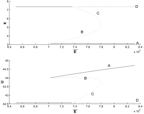
not positively correlated; that is, economic agents’ welfare at a fixed point with a high accumulation level can be lower than at a fixed point with a low accumulation level. Firstly, we assume: α = 0.8, β = 0.05, γ = 0.1, δ = 0.2, ε = 0.75,

a= 2.5,b= 0.1,d= 0.05,r = 0.1; in Fig. 4 we represent capital accumulation values k∗_{, evaluated at the fixed points A, B, C and D, as functions of the}

parameterE¯ (remember that E¯ is the endowment of the natural resource in the economy). The context we consider is that of Fig. 3, so, in the fixed pointAit holds that c2 = 0(i.e., the private good is not consumed as a substitute for the

environmental good) while inB, C andD we havec2 > 0; among these,D is

the fixed point where E = 0, that is where the natural resource is completely depleted.

6.4 6.6 6.8 7 7.2 7.4 7.6 7.8 8 8.2 8.4

x 105 3

4 5 6 7 8x 10

5

E

k

*

6.4 6.6 6.8 7 7.2 7.4 7.6 7.8 8 8.2 8.4

x 105 42.5

43 43.5 44 44.5 45

E

U

A B

C

D

A

B

C

D __

__

Fig. 4. Caseα= 0.8,β = 0.05,γ= 0.1,δ= 0.2,ε= 0.75,a= 2.5,b= 0.1, d= 0.05,r= 0.1.

Reachable fixed points (i.e., those having at least two negative eigenvalues) are indicated by continuous lines, the others by dotted lines. Note that, for suf-ficiently low values of E¯, only D is reachable; for sufficiently high values of

¯

consequence of a reduction ofE¯ (due, for example, to an exogenous shock) can be the convergence of the economy to a fixed point with a higher accumulation level.

In Fig. 4 we also represent the values assumed by the utility functionU at the fixed pointsA, B,C andD, as functions of the parameterE¯. Observe that the highest utility value is obtained at the fixed pointAwith the lowest accumulation level; the opposite holds for the fixed point D where the highest accumulation level is associated with the lowest utility level.

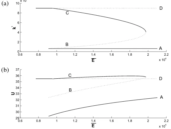
In Fig. 5 we modify the preceding example by assuming (coeteris paribus)

δ = 0.5. In Fig. 5a, we can see that only the fixed pointD(respectively, only the fixed pointA) is reachable ifE¯ is low enough (respectively, ifE¯is high enough). For intermediate values ofE¯, two fixed points are reachable:AandDorAandC. Note that the effects of an increase ofE¯ on the values ofk∗_{at the reachable fixed}

points are similar to those of the former example; however, in the latter example, we can see that inDandCthe utility function assumes values higher than inA; consequently, in this context, economic growth is desirable.

(a)

(b)

0.6 0.8 1 1.2 1.4 1.6 1.8 2 2.2

x 104 0

2 4 6 8 10x 10

4

E

k

*

0.6 0.8 1 1.2 1.4 1.6 1.8 2 2.2

x 104 29

30 31 32 33 34 35 36 37

E

U

__

__

A B

C

D

D C

B

A

These results are due to the fact that the productive activity of each agent also generates positive externalities on the productive activity of the others; con-sequently, the level of welfare obtained is the result of the interaction of both positive and negative effects deriving from the choices of each agent. In the former example, negative externalities overcome positive externalities; vice versa in the latter.

8 Hopf bifurcations

Our interest in the existence of periodic orbits is motivated by the fact that oscil-lations of the state variables kandE produce a reduction in welfare compared with a state of the economy where the values ofk andE are equal to the time averages ofkandE along the periodic orbit, if economic agents are risk-averse (see, e.g., [13]).

The existence of periodic orbits in thec2 = 0regime was analyzed in [22],

where a supercritical Hopf bifurcation was shown to give rise to a locally at-tracting periodic orbit (i.e., with a three-dimensional stable manifold). Let us now investigate, in thec2 >0regime, local bifurcations taking place at the equilibrium S = (k∗_{, c}∗

1, E∗), withE∗ >0, whenk∗varies in(k1, k2).

Case 1. Assumeα+δ _≤1andS is a repellor fork∗

belonging to a sub-interval

I of(k1, k2).

Then c∗1

k∗ is decreasing and ψ

′

(k∗

) < 0 inI. It follows that, when k∗

ap-proachesk2, generically a Hopf bifurcation occurs, as the real part of two complex

conjugate eigenvalues turns from positive into negative. In other words, fork∗

belonging to a suitable left neighborhood ofk₂,Shas a bi-dimensional stable and a one-dimensional unstable manifold.

Case 2. Assumeα+δ >1andSis an attractor fork∗_{belonging to a sub-interval}

I = (k3, k4)of(k1, k2).

Thenψ′_(k∗_)<0and c∗1

k∗ is decreasing inI. Furthermore, recalling d

′_:= d

a+1,

1₋α+α

d < δ <1−α+ α d′ +

(α+d′

)ε

(1₋α)d′,

It is easily seen thatk4=k2, if

1₋α+ α

d′ < δ <1−α+

α d′ +

(α+d′

)ε

(1₋α)d′,

whilek4 < k2, if

1₋α+α

d < δ <1−α+ α d′.

In the latter case, whenk∗_crossesk

4, one real negative eigenvalue becomes

posi-tive, passing through_∞, andShas a bi-dimensional stable and a one-dimensional unstable manifold ask∗

∈(k4, k2).

Furthermore it may happen thatk3 > km, wherekm = k0 orkm = k1, in

Cases 1 and 2, respectively.

If this occurs, then, generically, a Hopf bifurcation takes place when k∗

crossesk3, asSbecomes an attractor from a saddle with a one-dimensional stable

manifold.

Case 3. Consider the case

δ >1₋α+ α

d′ +

(α+d′

)ε

(1₋α)d′. (20)

Then no bifurcation occurs in the possible intervalJ_⊆(k1, k2), whereψ′(k∗)<0.

In such an interval S has a one-dimensional stable and a bi-dimensional unstable manifold.

If, furthermore, γ < σ < abβ + γ, then, passing through k₀ (recall

ψ′_(k

0) = 0), one real eigenvalue changes sign: it may turn either from positive

into negative or vice versa.

Case 4. Finally a generic Hopf bifurcation can take place in the possible interval

H _⊆(k1, k2), whereψ′(k∗)>0.

Example. In the following numerical example (12) and (20) hold and(k1, k2)is

divided into three sub-intervals: (k₁, kh),(kh, k0),(k0, k2). Ask∗ ∈ (k1, kh),S

is a repellor. Then at kh a Hopf bifurcation occurs andS has a bi-dimensional

stable and a one-dimensional unstable manifold fork∗

∈(kh, k0).

Finally, whenk∗

crossesk₀, a real negative eigenvalue becomes positive and

S has a one-dimensional stable and a bi-dimensional unstable manifold ask∗

∈

The example is

α= 1

2, a=b=β = 1, d= 4, δ= 2, r = 1 2√65, α₋ε sufficiently small,

γ = (α₋ε)2.

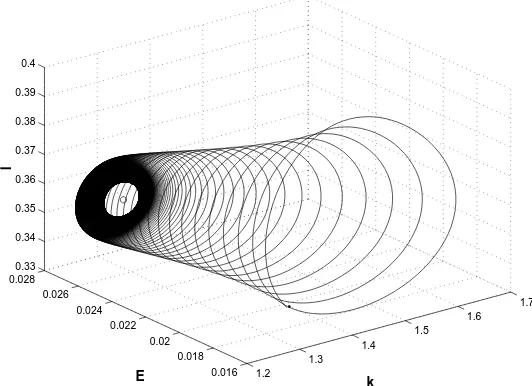
In this section we have shown all the Hopf bifurcations which can occur in our model. In Fig. 6, a locally attractive periodic orbit and one orbit approaching it are plotted . In such a case, given the initial values ofkandE[near enough to the projection of the orbit on the(k, E)plane], there exists a continuum of initial values ofλ(or, alternatively, of c₁ orc₂) by which the economy can reach the periodic orbit. Consequently, an indeterminacy problem occurs.

1.2 1.3

1.4 1.5

1.6 1.7

0.016 0.018 0.02 0.022 0.024 0.026 0.028

0.33 0.34 0.35 0.36 0.37 0.38 0.39 0.4

k

•

E

l

Fig. 6. Attracting limit cycle in caseα = 0.8, β = 0.05, γ = 0.1, δ = 0.2, ε= 0.75, a= 2.5, b= 1, d= 0.05, r= 0.1.

9 Behavior of orbits for high values ofE¯

Theorem 6. WhenE¯is sufficiently high, orbits starting in the regionc2 >0enter

Proof. To this end, let us replace, first, the variables(k, λ, E)in system (7)–(9) by(l, c₁, E), wherel _∈ (0,1)is defined by (4) andc₁ = 1_λ. It follows from (4) thatk=dl_α1₍₁−₋α−_l)δc1

1

1−α+ε

.

Hence we get, after simple steps,

˙

c1 =c1

(1₋α)α

d

α−ε

1−α+ε l ε+δ

1−α+ε(1−_l) α₋ε

1−α+ε

c

α−ε

1−α+ε

1

−r

. (21)

This impliesc˙₁<0, if

c₁> cM₁ :=1−α

r

1−α+ε α₋ε

max

l∈(0,1)l

ε+δ α−ε(1−l)

= α(α−ε)

d(α+δ)

_1−α

r

1−α+ε α−ε ε+δ

α+δ

ε+δ α−ε

.

(22)

Now assume

¯

E > b(a+ 1)cM₁ , if bβ > γ, (23)

¯

E > γ

β(a+ 1)c

M

1 , if bβ ≤γ. (24)

It follows, in particular, as is easily checked, that no equilibrium exists in the

c₂ >0regime.

Furthermore, consider an orbit starting in the region c2 > 0, i.e., such that ac1(0)> E(0)_b .

Due to (21) and (22), and since no equilibrium exists whenc₂ >0, there is a timet1such that either

c2(t1) = 0 (25)

or

c1(t)≤cM1 whent≥t1. (26)

Ifc2(t1) >0, thenE˙(t1) >0, because of assumptions (23) and (24). Hence E

increases, by a speed bounded away from zero, whereasc1 ≤cM1 . Consequently

there exists a timet2 > t1such that

Finally, we can chooset¯, ¯t _≥ ti, i = 1,2, in such a way that c1(t) ≤ cM1 for t_≥t¯andc₂(t) = 0fortbeing in some right neighborhood of¯t(in the particular case _αα_+d = _αε+₊δ_δ, the (22) value of cM₁ can be replaced by any slightly larger value). Otherwise, effectively, E would continue to increase, in line with our assumptions, in the regionc2>0, until we would obtain

E > abcM_{1 ≥}abc1,

thus contradicting the conditionc2 >0.

Now it is easily checked that assumptions (23) and (24) imply that, in the

c2 = 0regime,E˙(t)≤0,t≥¯t, requiresE(t)to be larger thanabcM1 . However, in

this case, the orbit would never cross back the planeac₁ = E_b. Therefore, should the orbit keep crossing such a plane forwards and back , i.e., moving indefinitely from the regime c2 > 0 to the regimec2 = 0and vice versa, E˙(t) would be

positive and bounded away from zero ast _≥¯t, until at some time, in thec₂ >0

regime,

E > abcM_{1 ≥}abc1,

yielding a contradiction.

Hence we can choose the previous¯tas the time at which the orbitentersinto and thenremainsin thec₂ = 0regime.

10 Conclusions

In order to better evaluate the relevance of the results obtained by our work, it may be useful to bear in mind what the dynamics of economic growth would be if the private good produced in the economy could not be consumed by the economic agents as a self-protection device against the deterioration of the environmental resource. In this case, whatever the values of E and k, the dynamics of the economy would only be described by the dynamics with c2 = 0, that is there

fixed point with c2 = 0, we can also have another three fixed points at which

we havec₂ >0; in these the levels of capital accumulation and consumption are higher than in the fixed point withc2= 0.

We have showed that the fixed point with c2 = 0 exists only if, coeteris

paribus, the endowment of the environmental good E¯ is sufficiently high and the negative impactγ of average consumption on the environmental good is suf-ficiently low; however, the values of E¯ and γ play no role in its stability pro-perties. Furthermore, we have showed that when E¯ is sufficiently high, orbits starting in the regionc2 > 0enter and remain, after a finite time, in the regime c2 = 0. Consequently, for high values ofE¯, the dynamics of the economy rule

out definitively substitutive consumptions.

WhenE¯is lower, dynamics become more interesting; in particular, bi-stable regimes can occur where the economy may reach the fixed point (or a periodic orbit) wherec2 = 0or a fixed point (or a periodic orbit) wherec2 >0depending

on the initial values of E and k. Furthermore, when α+δ > 1, there is the possibility of three reachable fixed points (see remark concerning Subcase 1 in Section 6); for example, it can happen that the fixed point withc2= 0is attractive,

the one withE > 0,c₂ > 0 andψ′_(k∗_{) > 0is a saddle with a bi-dimensional}

stable manifold and the fixed point satisfyingE > 0,c2 > 0andψ′(k∗) < 0is

attractive.

The complexity of the scenario described above is enhanced if we consider that indeterminacy can occur; in this case, even economies characterized by iden-tical technologies, preferences and endowments of environmental goods, starting from the same initial values ofE andk, may follow different growth dynamics choosing different initial values of λ (the multiplier associated with the state variablek). Note that the dynamics we have analyzed can have an attracting fixed point in the regimec₂ >0and a (reachable) saddle point inc₂ = 0; this implies that self-protection choices can cause indeterminacy.

(and, consequently, the level of consumption of the private good) and economic agents’ welfare. In particular, at the fixed point where capital accumulation is relatively low andc2 = 0, welfare may be greater than in the other fixed points.

Section 7 gives a numerical example where economic growth is undesirable and shows, by another example, that increasing (coeteris paribus) the value of the parameter δ (the exponent of average labour input), desirable economic growth can be obtained. These results are due to the fact that the productive activity of each agent also generates positive externalities on the productive activity of the others; consequently, the level of welfare obtained is the result of the interplay between positive and negative effects deriving from the choices of each agent. In the former example, negative externalities overcome positive externalities; vice versa in the latter.

The basic lesson emerging from the analysis of the model is that the aggregate level of consumption of the private goods is a distorted index of individuals’ welfare. This paper suggests that economic growth policies which are capable of achieving their goals, but at high environmental costs, should be treated with great caution. Economic policies ought to guarantee the growth of the values of appropriate welfare indices, which take into consideration not only the level of aggregate consumption but also that of environmental degradation and of self-protection consumption.

their models of consumption. By reducing the acoustic and atmospheric pollution, such measures contribute greatly to extending the offer of free access sites where the citizens can enjoy their free time, and therefore contribute to reducing self-protective consumption. In general, on the basis of the results of our model, it would appear desirable for the public administration to identify and classify all the activities which may generate self-protective consumption, with reference to the types of entity involved (individuals, firms, public sector), the sites in which such activities are carried out and, finally, the possible solutions which can be offered by the public sector. The public administrators are the only entities which can implement efficacious intervention in that, as the model shows, even perfectly rational individuals may select inefficient models of consumption.

Appendix A

Fromc˙1= 0and

˙

E

E −γk˙ = 0it follows E∗

= ¯E₋ γr

(1₋α)βk

∗_.

(A.1)

Then, fromE˙ = 0,

c∗

1 =c∗1 =

¯

E

(a+ 1)b +

(bβ₋γ)r

(a+ 1)(1₋α)bβk

∗_.

(A.2)

SinceE∗_{, c}∗

2 >0, (A.1) and (A.2) imply

(1₋α)β

(abβ+γ)rE < k¯

∗

< (1−α)β γr E.¯

Furthermorec˙₁ = 0and ∂H

∂l = 0imply dl∗

1₋l∗ =

αr

1₋α k∗

c∗

1

(A.3)

and, puttingA=lδkǫinc˙1 = 0,

(l∗

)α+δ= r 1₋α(k

∗

From (A.3) and (A.4) it follows

(1₋α)d αr c

∗

1+k∗=

_1−α

r

1

α+δ

(k∗

)αε++δδ

and, finally, from (A.2) we get (11).

Appendix B

It is easily computed that

A= (1−α+ε)(α+δ)

dr α(1−α)

c∗

1

k∗

r

1−α −(α+δ−1) d α

c∗

1

k∗

+ (1₋α+ε) r 1₋α,

B = −(α+δ)

dr α(1−α)

r

1−α−(α+δ−1) d α c∗ 1 k∗ .

Recalling the form ofψ(k∗_{)in (11), one obtains}

det J(S)= −(α+δ)βdrc

∗

1E∗ψ′(k∗) αβk∗

r

1−α −(α+δ−1) d α c∗ 1 k∗ . (B.1) Appendix C

Lettingα+δ_≤1, (B.1) implies

det J(S)ψ′

(k∗

)<0, when ψ′

(k∗

)₆= 0.

Hence, if ψ′

(k∗

) < 0, detJ(S) > 0 and the proposition follows. Then, let

ψ′_(k∗_{)>0and consequentlydetJ(S)<0.}

Denote bygik,i, k= 1,2,3, the entries ofJ(S). Observe, firstly, that

g11+g22=

ε(α+δ) dr α(1−α)

c∗

1

k∗

r

1−α + (1−α−δ) d α

c∗

1

k∗

+ (1₋α+ε) r

1₋α >0. (C.1)

The characteristic polynomial ofJ(S)is

where

H=g11g22+g33(g11+g22)−g12g21. (C.3)

From elementary algebra a cubic polynomial

λ3+aλ2+bλ+c (C.4)

has all non-positive real part roots, if and only if

a, b, c, ab₋c_≥0. (C.5)

It follows from (C.1) that

tr (J) =g11+g22+g33≤0impliesg33<0,

whileH _≥ 0, beingg₁₁g₂₂,g₃₃(g₁₁+g₂₂),g₁₂ <0, requiresg₂₁ >0. Finally the conditionab₋c_≥0means_|detJ_{| ≤}H_|trJ_|. Through simple calculations, though,

|detJ_|=_|g33|(g11g22−g12g21)

> _|g33| −(g11+g22) g11g22+g33(g11+g22)−g12g21=|trJ|H.

Hence we arrive at a contradiction.

We can conclude that, whenψ′_(k∗_{)>0,J(S)has only one eigenvalue with}

negative real part, and therefore negative.

Appendix D

Let us show that for any valueα+δ_≤1it is possible to have a repellorS, in the

c2 >0regime, withE∗ >0andψ′(k∗)<0.

Letγ < σ < abβ+γ, so that there existk0 ∈(k1, k2)satisfyingψ′(k0) = 0.

CallS0 the corresponding equilibrium.

In order that S be a repelling equilibrium for k∗

lying in a suitable right neighborhood ofk₀, it suffices that the two non-zero eigenvalues of J(S₀)have positive real part.

The non-zero roots ofP0(λ)have positive real part, if and only if

trJ0, H0 >0. (D.1)

It is easy to check that (D.1) is verified, whenα₋ε >0is sufficiently small and, furtherly,

γ = 2(α₋ε), β =d=α₋ε, b= 1,

a >2(ǫ+δ)

α ,

(1₋α)(ε+δ)

r(α+δ) >1.

References

1. A. Antoci, S. Bartolini. Negative externalities as the engine of growth in an evolutionary context, working paper No. 83.99, Fondazione ENI Enrico Mattei, 1999.

2. A. Antoci, S. Bartolini. Negative externalities, defensive expenditures and labor supply in an evolutionary game, Environment and Development Economics, 9, pp. 591–612, 2004.

3. S. Bartolini, L. Bonatti. Environmental and social degradation as the engine of economic growth,Ecological Economics,43, pp. 1–16, 2002.

4. S. Bartolini, L. Bonatti. Undesirable growth in a model with capital accumulation and environmental assets,Environment and Development Economics,8, pp. 11–30, 2003.

5. R. Hueting. New scarcity and economic growth. More welfare through less

production,North Holland, 1980.

6. C. Leipert. National income and economic growth: the conceptual side of defensive expenditures,Journal of Economic Issues,31, pp. 843–856, 1989.

7. C. Leipert, U.E. Simonis. Environmental protection expenditures: the German example, Rivista Internazionale di Scienze Economiche e Commerciali, 36, pp. 255–270, 1989.

8. J.R. Vincent. Green accounting: from theory to practice,Environment and

Develop-ment Economics,5, pp. 13–24, 2000.

9. J. Bird. The transferability and depletability of externalities,Journal of

10. J.F. Shogren, T.D. Crocker. Cooperative and non-cooperative protection against transferable and filterable externalities,Environmental and Resource Economics,1, pp. 195–213, 1991.

11. F. Hirsch.Social limits to growth,Harvard University Press, 1976.

12. A. Antoci. Negative externalities and growth of the activity level, working paper No. 9308 of the MURST Research ProjectNonlinear Dynamics and Applications to

Economic and Social Sciences,University of Florence, 1996.

13. J. Benhabib, R.E.A. Farmer. Indeterminacy and sunspots in macroeconomics,

Handbook of Macroeconomics, North Holland, 1999.

14. A. Antoci, P.L. Sacco, P. Vanin. On the Possible Conflict Between Economic Growth and Social Development, in: Economics and Social Interaction: Accounting for

Interpersonal Relations,B. Gui, R. Sugden (Eds.), Cambridge University Press, 2005

(forthcoming).

15. R.M. Auty. The political economy of the resource-driven growth, European

Economic Review,45, pp. 839–846, 2001.

16. K. Matsuyama. Agricultural productivity, comparative advantage, and economic growth,Journal of Economic Theory,58, pp. 317–334, 1992.

17. F. Rodriguez, J.D. Sachs. Why do resource-abundant economies grow more slowly?,

Journal of Economic Growth,4, pp. 277–303, 1999.

18. J.D. Sachs, A.M. Warner. The big push, natural resource booms and growth,Journal

of Development Economics,59, pp. 43–76, 1999.

19. J.D. Sachs, A.M. Warner. The curse of natural resources,European Economic Review,

45, pp. 827–838, 2001.

20. A. Antoci. Environmental resources depletion and interplay between negative and positive externalities in a growth model, working paper No. 9.05, Fondazione ENI Enrico Mattei, 2005.

21. R.J. Barro, X. Sala-i-Martin.Economic Growth,McGraw-Hill Inc., 1995.

22. A. Antoci, L. Brugnano, M. Galeotti. Oscillations, sustainability and indeterminacy in a growth model with environmental assets, Nonlinear Dynamics: Real World