Enhanced Software Quality Metrics for Fault Prediction
in Object Oriented Components using SVM Classifier
C.Neelamegam
Sri Venkateswara College of Computer Applications and Management
Coimbatore,India.
M.Punithvalli
Sri Ramakrishna Engineering College Coimbatore,Tamilnadu,
India.
ABSTRACT
Software quality metrics are defined as methods for quantitatively determining the extent to which an object oriented (OO) software process possess a certain quality attribute. Increase in software complexity and size is increasing the demand for new metrics to identify flaws in the design of OO system. This demand has necessitated this study to focus on adopting new metrics for measuring class complexities, for which established practices have yet to be developed. The proposed system works in two stages. The first stage presents new software metrics for measuring class complexity and the second stage analyzes the use of SVM classifier to predict faulty modules. Four new metrics, namely, Class Method Flow Complexity Measure, Friend Class Complexity Metric, Class Complexity from Inheritance and Class Complexity from Cohesion Measure, are proposed. These metrics, combined with 20 existing metrics, are used during prediction using SVM. The performance of prediction system is analyzed in terms of accuracy, precision, recall and F Measure. The experimental results showed positive improvement in the performance of prediction with the inclusion of the proposed metric and SVM classifier.
Keywords
Class Complexity, Object Oriented Quality Metrics, Software Fault Prediction, Support Vector machine.
1.
INTRODUCTION
Software quality metric is defined as methods for quantitatively determining the extent to which a software process, product or project possess a certain quality attribute. They are used to measure software engineering products (design, source code, etc), processes (analysis, design, coding, testing, etc.) and professionals (efficiency or productivity of an individual designer). The main aim of these techniques is to accurately identify and/or predict faulty modules which have direct impact on the three pillars of software product, namely, time, cost and scope. In the past few decades, software industries have realized the potential of using metrics to assess and improve the performance of developed projects, reduce time-to-market and improve customer satisfaction. Quality metrics can be categorized into process and product metrics.
Process metrics focus on improving the software development and maintenance processes, while product metrics improve software products by reducing the complexity of design, size and increase usability. In general, they should, be simple to understand, be precisely defined, decrease the influence of manual intervention, be cost effective and be informative. Techniques and methods that identify and predict faults using these quality metrics has gained wide acceptance in the past few decades ([6], [7]).
Existing metrics for fault module detection include CK metrics and Mood metrics along with traditional general metrics like simple metrics and program complexity measures. Traditional metrics do not consider OO paradigms like inheritance, encapsulation and passing of message and therefore do not perform well with fault prediction. The OO metrics have been developed specifically to analyze the performance of OO system. But, the increase in software complexity and size is increasing the demand for new metrics to identify flaws in the design and code of software system. This demand has necessitated the researchers to focus on adopting new metrics for which established practices have yet to be developed. This paper focus on such needs through the development of four metrics for OO design. In particular, this work analyzes metrics for measuring class complexities that can be used as a medium to identify design defects. For this purpose, four metrics based on flow of information, friend class/function, inheritance and cohesion are proposed. To analyze the performance of these metrics on fault module detection, the study proposes the use of SVM classifier.
The rest of the paper is organized as follows. Section 2 presents the four proposed metrics to calculate the complexity of the class. The methodology used by proposed prediction based classifier that uses existing and proposed metrics to predict faulty class is presented in Chapter 3. Several experiments were conducted to analyze the performance of the proposed metrics and SVM classifier to predict faulty modules. The results are presented and discussed in Section 4. Section 5 concludes the work with future research directions.
2.
PROPOSED METRICS
This section discusses four proposed complexity metrics and with all the metrics a high value denotes high excessive functional complexity and indicates serious design flaws that requires extensive testing and redesigning.
2.1
Class Method Flow Complexity
Measure (CMFCM)
According to [14], the module complexity can be calculated as in Equation (1).
CMFCM = (Fan-In * Fan-Out)2 + Code Length (1) (1)
It is known fact that in object-oriented systems, the private data (internal data) of an object cannot be directly accessed by other objects and therefore programmers use parameter passing and return values. The Fan-In (FI) and Fan-Out (FO) measures for a method ‘m’ should taken into consideration these values and can be calculated using the following Equations (2) and (3).
FI =1+ Nm1 + (NIP+ NPV+ NPU+ NLV + NGVR) + f( ) (2) (2)
FO = = 1 + Nm2 + (NOP+ NGVW) + f( ) (3) (3)
where Nm1 is the number of objects called, Nm2 is the number of objects that call this method, NIP is No. of input parameters, NPV is the No. of protected variables, NPU is No. of public variables, NLV is the No. of Local variables, NOP is the number of parameters written to, NGVR and NGVWare number of global variables read and written to and f( ) is a function which returns a value 1 if method ‘m’ returns a value, zero otherwise.
Another property that has to be considered while considering OO systems is the coupling among entities. The Coupling Among Entities (CAE) is calculated as the sum of indirect coupling metric and direct coupling metric (Equation 4). CAE = DCM + IDCM (4) where
DCM=
m in Parameters of
No m in Methods of
No
C the in parameters of
No C in Methods of
No
. .
.
.
and ICM=Product of DCM of all methods in the length of two entities and C is the class and m is the method Consider, for example, a system with entity relationship as shown in Fig. 1.
Fig. 1 : Sample entity relationship diagram
In this scenario, a direct coupling exists between entities (Ent-1, Ent-2), (Ent-2, Ent-3) and (Ent-3, Ent-4), while there is no direct coupling between entities Ent-1 and Ent-4. This will produce a zero value to DCM(Ent-1, Ent-4). However, there is a path from Ent-1 to Ent-4 through Ent-2 and Ent-3, which can be used during the calculation of coupling measure. Here the length between the entities Ent-1 and Ent-4 is 3 and the Indirect Coupling Measure is calculated as DCM(Ent-1, Ent-2) * DCM(Ent-2, Ent-2) * DCM(Ent-3, Ent-4). Now, Equation (1) can now be rewritten as
CMFCM = (FI + FO) * CAE * MCL (5) Here, the multiplicative operator in the traditional complexity measure is replaced by an additive operator. This modification was done to accommodate coupling among entities computation. This has the added advantage of reducing computation complexity. In the equation, MCL is the module code length and is calculated using Equation (6). MCL = LOC + MLOC + CLOC + (CL * j) + BL (6)
where LOC is the line of codes with comments and blank lines, MLOC is the multiline of code which is calculated as LOC * number of separate statements in the same line, CLOC is the line of code that contain comments and is calculated as the sum of LOC and number of comment lines. CL * j expression denotes the number of lines that contain more than
one comment statement and BL denotes the blank lines. The proposed CMFCM metric is a method level metric.
2.2
Friend class complexity metric
(FCCM)
A friend class is defined as a function or method that can access all private and protected members of a class to which it is declared as a friend. While considering complexity measure for friend classes, the following characteristics have be noted. 1. On declaration of friend class, all member functions of the friend class become friend of the class in which the friend class is declared.
2. Friend class cannot be inherited and every friendship has to be explicitly declared.
3. The friendship relation is not symmetric
In the field of OO metrics for fault detection, studies on friend classes are minimum, inspite of its extensive usage ([8], [9]). Friend constructs are violation of encapsulation and will complicate a program, which in turn, makes debugging more difficult. Moreover, the task of tracking polymorphism also becomes more complex while using friend classes. According to Chidamber and Kemerer's principle only those methods which require additional design effort should be counted for metric measurement and inherited methods and methods from friend classes are not defined in the class and therefore, need not be included. However, it has been proved that the coupling that exists between friend classes increase fault proneness of a class [4]. These methods consider relationship and type of association between class attributes and methods and do not consider the relationship between friend attributes and external attributes. This section proposes a modified version, which considers this relationship and extends coupling metrics to use these friend metrics. Using these metrics, a new coupling measure to determine the class complexity is proposed.
Coupling measure can be either Direct Coupling (DC) or Indirect Coupling (IDC). DC here refers to the normal coupling factor, while IDC refers to coupling while friend functions or classes are used. Thus the new coupling factor is defined as a sum of DC and IDC (Equation 7).
CFNew = DC + IDC (7) DC is calculated using the method specified in Mood metric suite. The IDC of a class is calculated as average of Method IDC (MIDC) factor. The MIDC is modified to identify a factor called actual friend methods, which is introduced because generally, a friend class declaration grants access to all methods in a class but in reality only a few of these methods are actually called by other classes. The MIDC combined with this factor is calculated using Equation (8).
MC N
1
i GVR GVW GF PC V
N
N N N ) N (N
MIDC
MC
i i i i i
(8) where NGF is the number of global functions, NPC is the number of messages to other classes and NV is the number of references to instance variables of other classes and NMC is the number of actual methods in the class which is calculated as the difference between the number of methods (NM) and Number of Hidden Methods (NHM) in a class (Equation 9). Hidden methods are methods that cannot be called on an object of the class without the use of the friend construct.
Ent-1
Ent-2
Ent-3
NMC = NM – NHM (9) (9) The number of hidden methods is calculated as the number
of methods in a class that access hidden members of classes which declare the current class as a friend [12]. NHM is calculated as the sum of two measures. The first is the number the hidden methods belonging to other classes accessed by the class. This measure is called in this study as Number of EXternal Hidden Methods NHME. The second measure is the number of hidden methods that are invoked by other classes from the class. This measure is referred in this study as Number of Internal Hidden Methods NHMI. Thus NHM is calculated as
NHM = NHME + NHMI (10) Using the above metric, the complexity measure can be calculated by modifying Equation (5) as given below
FCCM = (FI + FO) * CFNEW * MCL (11) Again, this metric is a method level metric, where a high value indicates design flaws.
2.3
Class complexity from inheritance
(CCI)
Inheritance a powerful mechanism in OO programming provides a method for reusing code of existing objects or establishes a subtype from an existing object, or both. Inheritance metrics are used to analyze various aspects of a program in terms of depth, breadth in a hierarchy and its overriding complexity. It can be used to measure class complexity as a measure of data / method shared from ancestor classes. The class complexity while taking inheritance into consideration depends mainly on the inheritance type (single, multiple, multi-level inheritance). Apart from this, while calculating the class complexity with respect to inheritance, the complexity imposed by inherited methods and inherited attributes should also be considered. Thus the proposed CCI metric considers the individual complexity of a class while taking the properties of inheritance into consideration (ICC), inherited method complexity (IMC) and inherited attribute complexity (IAC) and is calculated using Equation (12).
CCI = ICC + IMC + IAC (12)
where ICC of a class i is calculated as
ICC = NA +
A
N
2
i i
ICC
(13)Here the ICC of the root of the inheritance tree is zero as it has no parent. Consider for example Fig.2 where, Class A1 and A2 are inherited from Class A and are examples of single class inheritance, while Class A3 is inherited from Class A1, which is inherited from Class A and presents an example of multi-level inheritance. Class A4 and A5 presents multiple inheritance as both are inherited from more than one class.
Fig. 2. Example class inheritance hierarchy
From the inheritance hierarchy presented in the figure, the ICC of Class A and Class B is zero, as both do not have
parent class. The ICC of Class A1 and A2 is calculated as 1 + 0 [ICC(Class A)] = 1. The ICC for Class A3 = 1 + ICC(Class A1) + ICC(Class A) = 1 + 1 + 0 = 2. Similarly, the ICC(Class A4) = 2 + ICC(Class A1) + ICC(Class A2) = 2 + 1 + 1 = 4, where 2 being the number of parents of A4. ICC(Class A5) = 2 + ICC(Class A2 ) + ICC (Class B) = 2 + 1 + 0 = 3.
The ICC measure thus takes into consideration the depth of the class in the inheritance hierarchy, number of parents of the class and their depth in the inheritance hierarchy along with the type of inheritance. The IMC is calculated as
IMC = (NPD * 1)+ (NDD * 2) + (NUD* 3) (14) where NPD is the number of primary data variables, NDD is the number of derived data variables and NUD is the number of user defined data type variables. The classification of data types is similar to the one proposed by [1], who defined PD as in-built data types like int, float and char, DD as in-built structures like arrays and UD as user designed structures which are formed by combining PD and DD. Examples for UD includes structure, union and class. As suggested by the same author, a cognitive weight of 1, 2 and 3 are used along with NPD, NDD and NUD respectively. These cognitive weights are assigned according to the cognitive phenomenon suggested by [17] which assigns weight for PD=1, DD=2 and UD=3.
Finally, IAC is calculated again by assigning cognitive weights to the control structures in the method. The control structures considered are sequence statements, branching statements, iterative statements and call statements. As suggested by [17]a value of 1, 2, 3 and 2 are assigned to these statements respectively.
2.4
Class complexity from cohesion
measure (CCCM)
Cohesion of a class describes how the methods of a class are related to each other. In general, a high cohesion is desirable as it promotes encapsulation, while a low cohesion indicates high likelihood of errors, design change and high class complexity. This section presents a metric to calculate class complexity through cohesion measure. Four types of cohesion methods are used, namely, Cohesion Among Attribute in a class Measure (CAA), Ratio of Cohesion Interactions (RCI), Cohesion Among Methods in a class (CAMC) and Normalized Hamming Distance (NHD) Metric. Here RCI, CAMC and NHD are calculated using steps as provided by [5], [2], [10]. The RCI considers the data to method relationship, the CAMC considers the method-method interactions The CCCM metric is a metric that is included in this study to measure the degree of similarity among methods while considering attribute usage.
CCCM = CCM + RCI + CAMC / 3 (15) 1) and CCCM is calculated as below. Calculate the number
of methods in a class, M (={m1, m2, …})
2) Calculate the number of instance variables in each method, Vi ({=V1,V2, V3, …}, i M)
3) Calculate number of methods using each instance from V, NVi, as (M Vi)-1. The value is 1 used to remove the attributes similarity dependency from the method it is declared.
Step 4 : Calculate CCCM as
xV ) 1 M (
N
M
1 i Vi
(16)
To understand the CCM measure, consider the following code snippet showing four methods of a class.
Class A Class B
Class A1 Class A2
Class A4
Class Sample
{ AddRecord() { int AccNo; char AccName []; float Balance;
…. } DeleteRecord() { int AccNo;
…. } SearchAccount() { int AccNo;
…. }
UpdateAcc() { int AccNo; float Balance; float WithDrawals; float Deposits;… }} From these codes, M=4 (={AddRecord, DeleteRecord, SearchAccount, UpdateAcc}) and V=5 (={AccNo, AccName,
Balance, WithDrawals, Deposits}).
NV1={AccNo,AccName,Balance, WithDrawals, Deposits} {AccNo, AccName, Balance}=3–1=2. Similar calculations for NV2, NV3, NV4 produces the values 0, 0 and 3 respectively. With these values the CCM measure can be calculated as CCCM = (2+0+0+3)/(4*(5-1))=5/16=0.3.
3.
Fault prediction using object oriented
metrics
The present study proposes the use of machine learning algorithm to analyze the performance of the proposed metrics in predicting design flaws in OO programs. The proposed method consists of four steps. (i) Selection of metrics (ii) Dimensionality Reduction (iii) Normalize the metric values and (iv) Implement prediction model. Here the prediction model is proposed as a binary classification task, where a module is predicted as either faulty (complex) or not-faulty (normal).
3.1
Selection of metrics
3.2
The four proposed metrics are
combined with twenty existing metrics
(Table 1) during fault prediction. The
selected existing metrics were chosen
because of their wide usage in fault
detection. Dimensionality Reduction.
The vital step in designing a classification model is the selection of a set of input metrics, which unless selected carefully will result in ‘Curse of dimensionality’ [3]. This phenomenon can be avoided by the use of dimensionality reduction procedure, which aims to reduce the number of input variables by removing irrelevant data and retaining only those data which are most discriminating.
Please use a 9-point Times Roman font, or other Roman font with serifs, as close as possible in appearance to Times Roman in which these guidelines have been set. The goal is to have a 9-point text, as you see here. Please use sans-serif or non-proportional fonts only for special purposes, such as distinguishing source code text. If Times Roman is not available, try the font named Computer Modern Roman. On a Macintosh, use the font named Times. Right margins should be justified, not ragged.
3.3
Title and Authors
The title (Helvetica 18-point bold), authors' names (Helvetica 12-point) and affiliations (Helvetica 10-point) run across the full width of the page – one column wide. We also recommend e-mail address (Helvetica 12-point). See the top of this page for three addresses. If only one address is needed,
center all address text. For two addresses, use two centered tabs, and so on. For three authors, you may have to improvise.
3.4
Subsequent Pages
[image:4.595.325.551.173.483.2]For pages other than the first page, start at the top of the page, and continue in double-column format. The two columns on the last page should be as close to equal length as possible.
Table 1. List of selected existing metrics
A
Simple metrics
1) LOC (Total number of lines) 2) BR (Number of methods)
3) NOP (Total Number of Unique Operators) 4) NOPE (Total Number of Unique Operands) 5) RE (Readability with Comment percentage) 6) VO (Volume)
B
Mood Metrics
1) MHF (Method hiding factor) 2) AHF (Attribute hiding factor) 3) MIF (Method inheritance factor) 4) AIF (Attribute inheritance factor) 5) PF (Polymorphism factor) 6) CF (Coupling factor)
C
Chidamber & Kemerer's Metrics
1) WMC (Weighted Methods per Class) 2) DIT (Depth of Inheritance Tree) 3) NC (Number of children)
4) COC (Coupling between object classes) 5) RC (Response for a Class)
6) LCM (Lack of Cohesion in Methods)
D
Program Complexity Measure
1) CC (Cyclomatic Complexity)
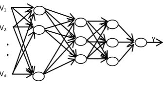
2) FI-FO(Fan-In Fan-Out) - Henry's & Kafura's) In the present study, Sensitivity Analysis of data is used for this purpose. Sensitivity analysis analyzes the importance of each input data in relation to a particular model and estimates the rate of change of output as a result of varying the input values. The resulting estimates can be used to determine the importance of each input variable [16]. This study adopts the Sensitivity Casual Index (SCI) proposed by [13]. SCI is calculated as follows. For a classifier having architecture as shown in Fig. 3, given a set of input Vectors, {Vi, n i 0}, where Vi belongs to the set of metric values collected from the input dataset with ‘d’ dimensions with single output Y = f(xi), the SCI for each input dimension is calculated using Equation (17).
n
1
i i i ij
j |f(V) f(V )|
SCI (17)
where |.| denotes absolute value and ij is a small constant
added to the jth component Vj of Vi.
3.5
Normalization
Fig. 3 : Classifier architecture
Further, normalization is performed to improve the training process of the classifier. Normalization is performed by estimating the upper and lower bounds for each metric value and then scale them using Equation (18).
) V min( ) V max(
) V min( V V
j j
j j
'
j
(18)
where
V
'j is the normalized or scaled value, min(Vj) andmax(Vj) are the maximum and minimum bounds of the metric ‘j’ from ‘n’ observations respectively. The result of normalization thus, maps each input value to a closed interval [0, 1].
3.6
Prediction model
The steps to build the prediction model are given below. Step 1 : Identify a classifier
Step 2 : Identify the feature vector to be used as input Step 3 : Partitioning method (Training and Testing sets) Step 4 : Train and test the classifier using n-fold
cross-validation method
The present study uses SVM for fault prediction. Input feature vector is created using metrics described in Section 2 and salient data is identified using the procedures described in Sections 3(A) and 3(B). The partitioning method used to separate the normalized, dimensionality reduced input data into training and testing set is the hold-out method. In the present study, two-thirds of the data is used during training and the rest of the one-third is used as testing set. Given a set of input data set, the Support Vector Machine (SVM) classifier marks each given input as belonging to one of two categories (faulty or not-faulty).
4.
EXPERIMENTAL RESULTS
The proposed fault-detection classifier systems using software metrics was developed using MATLAB and all the experiments were conducted on a Pentium IV machine with 4GM RAM. To analyze the applicability of SVM and the affect of the new metrics on fault identification, experiments were conducted with a commercial real-time C++ project from a software company in Coimbatore, India. Obliging to the privacy issues of the company, only the details of the software system from which metrics were calculated is mentioned here. The details were collected from various historical reports maintained by the company. The project contains around 45000 LOC with 1771 modules. After studying the error reports, around 1502 modules were found to have no errors (non-faulty modules) and the 269 were faulty modules.
The feature vector created has 24 dimensions (20 existing and 4 proposed). The feature vector V was created using the 24 software metric values (20 existing and 4 proposed). This vector was first normalized to an interval [0, 1] to ensure that all the 24 values have equal importance. Dimensionality
reduction was next performed on this set to select discriminating metrics by calculating SCI of each input dimension over the entire normalized dataset with =0.1. After calculation of SSI, the metrics were arranged in descending order of SSI and the top 15 metrics were selected. The resultant feature vector, after dimensionality reduced consist of LOC, BR, NOP, NOPE, RE, VO, MHF, PF, WMC, NC, RC, CMFCM, FCCM, CCI and CCCM. It can be seen that the resultant reduced dataset consists of only those metrics which has impact on complexity measure. Further, the SCI of all the four proposed metrics were high and came after all the simple metrics and WMC metric, which shows that the proposed metrics have relevant information with respect to the task of identifying faulty modules while considering complexity. The reduced dataset with 15 metrics is then divided into training (943 modules) and testing (628) datasets. Four performance metrics were used during evaluation. They are accuracy, precision, recall and F-measure, which are derived from the confusion matrix. A 10-fold cross validation method was used with all experiments. The performance of the SVM algorithm is compared with that of Back Propagation Neural Network (BPNN) and K-Nearest Neighbour (KNN) algorithms. For SVM classifier, the regularization parameter was set to 1, the kernel function used was Gaussian and bandwidth of the kernet was set to 0.5. For K-NN classifier, k was set to 3. For BPNN classifier, 2 hidden nodes with learning rate of 0.2 were used. ‘t’ test proposed by [15] was performed at 95 % confidence level (0.05 level) to analyze the significant difference between SVM and BPNN, SVM and KNN. This method was adopted because it is more suited for classifiers adapting 10-fold cross-validation method [11]. The traditional student ‘t’ test, method produces more false significant differences due to the dependencies that exists in the estimates.
Table 2 shows the performance based on Accuracy, Precision, Recall and F Measure and SD denotes the standard deviation. Sig denotes the significance status and a value ‘Yes’ denotes that there is a significance performance difference between SVM and the corresponding model, while a ‘No’ represents insignificant performance. A ‘+’ sign denotes that SVM has outperformed the corresponding classifier, while ‘– ’ sign denotes the opposite.
Table 2. Prediction performance
SVM BPNN KNN
Accuracy
Mean 91.6 77.38 85.29
SD 1.16 6.562 4.216
Sig Yes(+) Yes(+)
Precision
Mean 91.3 89.04 93.72
SD 0.04 0.016 0.029
Sig Yes(+) No (–)
Recall
Mean 99.9 80.12 91.09
SD 0 0.081 0.046
Sig Yes(+) Yes(+)
F Measure
Mean 0.95 0.874 0.901
SD 0.01 0.049 0.026
Sig Yes(+) Yes(+)
V1
V2
Vd
:
:
:
:
From the results, it is clear that the performance of SVM showed higher accuracy than both BPNN and KNN algorithm in terms of classification accuracy, as indicated by Yes (+) in significance column. While considering the precision of classifiers, SVM showed significant improvement with BPNN but was insignificant with KNN. However, the recall performance showed significant positive improvement when compared with both BPNN and KNN. The last parameter, F measure is the harmonic mean of precision and recall by taking both into consideration, The results show that both BPNN and KNN shows degraded performance when compared with SVM.
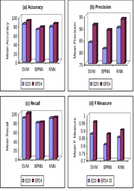
All these results show that SVM can be considered as the right candidate for identifying faulty modules. Fig. 4a to 4d shows the Mean accuracy, precision, recall and F measure while testing the classification algorithm with only existing 20 metrics (E20), existing and proposed metric (EP24 metrics). From the figures, it can be seen that the inclusion of the four new metrics has increased the performance of the classifiers. While comparing E20 and EP24 metrics, the EP24 metrics showed 7.58% accuracy improvement when compared with E20 metric set. Similarly, 8.12% and 9.69% efficiency gain with respect to precision and recall was seen with E24 metric set. All these results prove that the proposed metrics are efficient in identifying classes that have high complexity and flaws and therefore can be used by software industries to improve the design of OO software products.
0 20 40 60 80 100
M
e
a
n
A
c
c
u
r
a
c
y
SVM BPNN KNN (a) Accuracy
E20 EP24
75 80 85 90 95
M
e
a
n
P
r
e
c
is
io
n
SVM BPNN KNN (b) Precision
E20 EP24
0 20 40 60 80 100
M
e
a
n
R
e
c
a
ll
SVM BPNN KNN (c) Recall
E20 EP24
0.7 0.75 0.8 0.85 0.9 0.95 1
M
e
a
n
F
M
e
a
s
u
r
e
SVM BPNN KNN (d) F Measure
[image:6.595.56.271.369.674.2]E20 EP24
Fig. 4. Performance of proposed metrics
5.
CONCLUSION
This paper identified OO modules with faults in two stages. The first stage identified four new software metrics to measure class design complexity and second stage used SVM classifier to predict faulty modules. The four new metrics proposed are Class Method Flow Complexity Measure
(CMFCM), Friend Class Complexity Metric (FCCM), Class Complexity from Inheritance (CCI) and Class Complexity from Cohesion Measure (CCCM). These metrics were combined with 20 existing traditional metrics during prediction. Sensitivity index was used to select relevant metrics for classification after normalization. The experimental results showed positive improvement in the performance of prediction with the inclusion of the proposed metric and SVM classifier. In future, evaluation of the proposed metrics using criteria as suggested by [18] is planned. Moreover, the use of ensemble classification is also planned to increase the reliability and maintainability of the software product by increasing the accuracy of flaw module prediction.
6.
REFERENCES
[1] Arockiam, L. and Aloysius, A. (2011) Attribute Weighted Class Complexity: A New Metric for Measuring Cognitive Complexity of OO Systems, World Academy of Science, Engineering and Technology, 58,Pp. 808-813.
[2] Bansiya, J., Etzkorn, L., Davis, C. and Li, W. (1999) A class cohesion metric for object-oriented designs, Journal of Object-Oriented Program, Vol. 11, No. 8, Pp. 47-52.
[3] Bellman, R. (1961) Adaptive Control Processes, Princeton University Press.
[4] Briand, L.C., Devanbu, P.T. and Melo, W.L. (1997) An Investigation into Coupling Measures for C++, International Conference on Software Engineering, Pp.412-421.
[5] Briand, L.C., Morasca, S. and Basili, V.R. (1999) Defining and validating measures for object-based high-level design, IEEE Transactions on Software Engineering, Vol. 25, No. 5, Pp. 722-743.
[6] Catal, C and Diri, B. (2009) Investigating the effect of dataset size, metrics sets, and feature selection techniques on software fault prediction problem, Information Science, Elsevier, Vol. 179, Pp. 1040-1058.
[7] Chowdhury, I. and Zulkernine, M. (2011) Using complexity, coupling, and cohesion metrics as early indicators of vulnerabilities, Journal of Systems Architecture, Elsevier, Vol. 57, Pp. 294-313.
[8] Counsell, S. and Newson, P. (2000) Use of Friends in C++ Software: An Empirical Investigation. Journal of Systems and Software, Vol.53, No.1, Pp.15.21.
[9] Counsell, S., Newson, P. and Mendes, E. (2004) Design Level Hypothesis Testing Through Reverse Engineering of Object-Oriented Software, International Journal of Software Engineering, Vol.14, No.2, Pp.207.220.
[11] Dietterich, T. (1998) Approximate statistical tests for comparing supervised classification learning algorithms, Neural Computation, Vol. 10, Pp. 1895–1924.
[12] English, M., Buckley, J., Cahill, T. and Lynch, K. (2005) An Empirical Study of the Use of Friends in C++ Software, International Workshop on Program Comprehension, Pp. 329.332.
[13] Goh, T.H. and Wong, F. (1991) Semantic extraction using neural network modeling and sensitivity analysis, Proceedings of IEEE International Joint Conference on Neural Networks, Pp. 18–21.
[14] Henry, S.M. and Kafura, D. (1981) Software structure metrics based on information flow, IEEE Transactions on Sofware Engineering, Vol. SE-7, Pp. 510-518.
[15] Nadeau, C. and Bengio, Y. (2003) Inference for the generalization error, Machine Learning, Vol. 52, Pp.239– 281.
[16] Saltelli, A., Chan, K. and Scott, E.M. (2000) Sensitivity Analysis, John Wiley & Sons.
[17] Wang. Y, (2002) On Cognitive Informatics, IEEE International Conference on Cognitive Informatics, Pp. 69-74.
[18] Weyuker. E.J. (1988) Evaluating Software Complexity Measures, IEEE Transactions on Software Engineering,