Improved Edmond Karps Algorithm for Network Flow
Problem
Chintan Jain, Deepak Garg
Thapar University, PatialaABSTRACT
Network Flow Problems have always been among the best studied combinatorial optimization problems. Flow networks are very useful to model real world problems like, current flowing through electrical networks, commodity flowing through pipes and so on. Maximum flow problem is the classical network flow problem. In this problem, the maximum flow which can be moved from the source to the sink is calculated without exceeding the maximum capacity. Once, the maximum flow problem is solved it can be used to solve other network flow problems also. The FORD-FULKERSON algorithm is the general algorithm which can solve all the network flow problems. The improvement of the Ford Fulkerson algorithm is Edmonds-Karp algorithm which uses BFS procedure instead of DFS to find an augmenting path. The modified Edmonds-Karp algorithm is designed to solve the maximum flow problem in efficient manner.
Keywords
Edmonds-Karp algorithm, Maximum flow problem, Residual graph, Ford-Fulkerson method.
1.
INTRODUCTION
The maximum flow problem is to find the max. flow that can be sent through the arc of the network from some specified node source (s) to specified node sink (t) and a capacity
function that maps edges to positive real numbers, u: E |→ R+. Maximum flow involves a directed network with
arc carry flow; the relevant parameters are arc capacity and flow. [3,9]
Definitions and Notation of Maximum Flow Problem: Suppose G (V, E) is a finite directed graph in which every edge (u, v) ϵ E has a non-negative, real-valued capacity c (u, v). If (u, v) ϵ E, we assume that c (u, v) = 0. We distinguish two vertices: a source s and a sink t. A flow network is a real function f: V×V → R with the following three properties for all nodes u and v:
Capacity constraints:
f(u,v) ≤ c(u,v). The flow along an edge cannot exceed its capacity.
Skew symmetry: f(u,v) = -f(u,v). The net flow from u to v must be the opposite of the net flow from v to u
Flow conservation:
𝐟 𝐮, 𝐰 = 𝟎
𝐰 ϵ 𝐯 , unless u = s
or u = t. The net flow to a node is zero, except for the source, which "produces" flow, and the sink, which "consumes" flow.
Residual Network: The residual capacity of an edge is cf (u, v) = c (u, v) - f (u, v). This defines a residual network
denoted Gf (V, Ef), giving the amount of available capacity. In short residual network is nothing but the remaining network i.e. it shows that how much more flow can be sending on the network. [4]
Previously There has been a lot of work on maximum flow problems. Different improvements has been suggested by different researchers [1,2,6,7,8].
2.
PROBLEM DEFINITION
Suppose one pipeline system is there in Mumbai to supply water in different areas of Mumbai. The pipeline between any two areas has a stated capacity in gallons per hour, given as a maximum flow at which water can flow through the pipe between those two areas. Now, suppose we want to supply water from the source area, says A to the sink area, say I and water passes through 7 other areas before reaching from source to sink. Suppose these 7 areas are B, C, D, E, F, G, H and pipeline between any two areas has defined capacity. So, the problem is to calculate the maximum amount of water which can flow from A to I. Output is the maximum amount of water in gallons per hour which can flow from A to I.
3.
METHODOLOGY
The following steps are carried out to solve the problem.
First of all, the problem is converted into directed graph by representing area as a vertex of the graph and pipeline between any two areas as an edge of the graph. The capacity of the pipeline in gallons per hour is represented as capacity of an edge in units. Then new modified algorithm of the existing algorithm is designed. After this the problem is solved using both algorithms and comparison is done between them. Finally, the problem is implemented using implementation code of the new algorithm to achieve the desired outputLet the graph G = (V, E)be a flow network with source s, sink t, and an integer capacity c (u, v) on each edge(u, v) ϵ E.
Let C = max
u,v ϵ Ec(u, v).
4.
PROBLEM DESCRIPTION
4.1
CONVERTING THE PROBLEM
INTO GRAPH
Table 1. Defined capacities of each pipeline between two areas
Source Area
Destination Area
Capacity (gallons/hour)
A B 34
A B 20
A E 35
B D 20
B E 8
C E 8
C F 15
D F 10
D G 22
D H 18
E D 35
E F 15
F H 35
G I 48
H G 20
H I 30
[image:2.595.101.224.400.560.2]Now, following correspondence between areas and vertices is used to make a graph.
Table 2. Correspondence between areas and vertices
Area Vertex
A S
B 1
C 2
D 3
E 4
F 5
G 6
H 7
I T
So, the initial graph corresponding to the tables 1 and 2 is as follows.
20 22
34 8 35 48
35 10 18 20
15 20 8 30
[image:2.595.314.543.489.756.2]15 35
Fig 1: The initial flow network corresponding to the problem to be solved
Now the modified EDMONDS-KARP-METHOD is given below which can be used to compute a maximum flow in G. Algorithm I MOD_EDMONDS-KARP (G, s, t)
(1) for each edge (u, v)ϵ E[G] (First initialize the flow f to 0) (2) do f[u, v] ← 0
(3) f[v, u] ← 0 (4) C ← max
u,v ϵ Ec(u, v) (5) I ← 2 log2C
(6) while I ≥ 1
(7) do while there exists an augmenting path pfrom sto t in the residual network Gfof capacity atleast I (8) doc f (p) ← min {c f (u, v) ∶ (u, v) is in p}
(9) for each edge (u, v) in p
(10) do f u, v ← f u, v + c f(p)
(11) f u, v ← −f[u, v] (12) I = I 2
(13) return f
4.2
SOLUTION USING MODIFIED
EDMONDS-KARP ALGORITHM
Now, the maximum capacity of the graph is 48. So, the value of the variable Cin the above algorithm will be 48.
So,2 log2C = 32, which will be value of the variable I in the 1st iteration of the algorithm.
1st Iteration: I = 32. So, the augmenting path with capacity at least 32 will be searched by the Breadth First Search procedure. But, there is no augmenting path with capacity at least 32. So, no flow will be added to the initial flow of the graph which is 0.
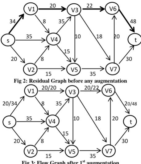
2nd Iteration: I = I 2 = 32 2 = 16. So, now the augmenting path with capacity at least 16 will be searched by the same BFS procedure in the residual graph which is given below in Fig 2 corresponding to the initial graph. The augmenting path will be searched till path with capacity at least 16 is found in the graph. Now, in the consecutive figures, the left side figure shows the residual graph and the right side figure shows the corresponding flow in the graph.
20 22
34 8 35 48
35 10 18 20 15 20 8 30
15 35
Fig 2: Residual Graph before any augmentation
20/20 20/22
20/34 8 35 20/48
35 10 18 20
15 20 8 30
15 35
Fig 3: Flow Graph after 1st augmentation
V6
V3
V1
s
V2
V4
V5
V7
t
V6
V3
V1
s
V2
V4
V5
V7
t
V6
V3
V1
V1
s
V2
V4
V5
V7
[image:2.595.52.283.600.725.2]Whenever the augmenting path is to be found in the graph, if there are more than 1 path satisfying the capacity criteria, then the path is determined by BFS procedure on the basis of sequential ordering of the vertices and corresponding edges which has been given as input.
1st augmentation: So, the augmenting path found in 2nd iteration is s-v1-v3-v6-t with capacity 20. So, the initial flow is augmented by 20 units and the flow in the graph is shown in the Fig 3 giving maximum flow value f = 20. The residual graph after 1st augmentation is shown below
20 2
20
14 20 8 35 20 28 35 10 18 20
15 20 8 30
15 35
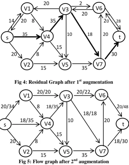
Fig 4: Residual Graph after 1st augmentation
20/20 20/22
20/34 8 18/35 20/48
18/18 18/35 10 20 15 20 8 18/30
[image:3.595.315.546.72.197.2]15 35
Fig 5: Flow graph after 2nd augmentation
2nd augmentation: Now, again there is a path with capacity at least 16 and the path found in the same 2nd iteration is s-v4-v3-v7-t with capacity 18. So, the maximum flow is augmented by 18 units and the flow in the graph is shown in the above Fig 5 giving maximum flow value f = 20 + 18 = 38. Now, there is no path with capacity at least 16.
Same procedure will be followed until variable I becomes <1.
3rd Iteration: I = I 2 = 16 2= 8 So, now the augmenting path with capacity at least 8 will be searched. The residual graph after 2nd augmentation is shown
20 2
20
14 20 8 17 20 28 17 18
10 18 20 18
15 12 20 8 18
15 35
Fig 6: Residual Graph after 2nd augmentation
20/20 20/22
20/34 8 18/35 20/48
18/18 18/35 10 20
15 12/ 20 8 30/30
[image:3.595.55.281.188.478.2]12/15 12/35
Fig 7: Flow graph after 3rd augmentation
3rd augmentation: The augmenting path found in 3rd iteration is s-v2-v5-v7-t with capacity 12. So, the maximum flow is augmented by 12 units and the flow in the graph is shown in the Fig 7 giving maximum flow value f = 38 + 12 = 50. The residual graph after 3rd augmentation is shown below
20 2
20 28
14 20 8 17 18 20 17
10 18 20 18
8 8 15
12 30
3 23
[image:3.595.325.544.295.422.2]
12 12
Fig 8: Residual Graph after 3rd augmentation
20/20 20/22
20/34 8 18/35 35/48
18/18 33/35 10 15/20
8 12/ 20 15/15 30/30
[image:3.595.318.543.299.574.2]12/15 27/35
Fig 9: Flow graph after 4th augmentation
4th augmentation: Now, again there is a path with capacity at least 8 and the path found in the same 3rd iteration is s-v4-v5-v7-v6-t with capacity 15. Maximum flow value f = 50 + 15 = 65. Now, there is no path with capacity at least 8.
4th Iteration : I = I 2 = 8 2 = 4. Now the augmenting path with capacity at least 4 will be searched. The residual graph after 4th augmentation is shown below
V6
V3
V1
V1
s
V2
V4
V5
V7
t
V6
V3
V1
s
V2
V4
V5
V7
t
V6
V3
V1
V1
s
V2
V4
V5
V7
t
V6
V3
V1
s
V2
V4
V5
V7
t
V6
V3
V1
V1
s
V2
V4
V5
V7
t
V6
V3
V1
s
V2
V4
V5
V7
[image:3.595.60.278.609.733.2]20 2
20 13 14 8 17 20 18 35
2
10 18 5 15 33
8 8 15 30 12 3 8
12 27
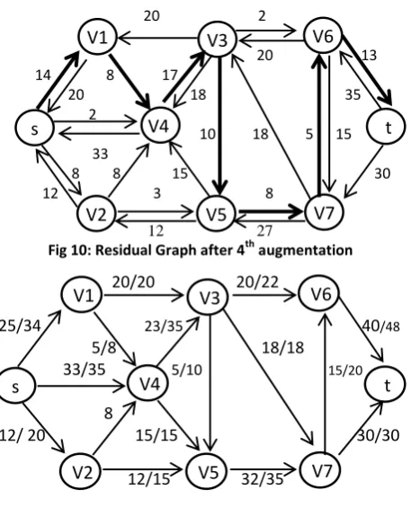
Fig 10: Residual Graph after 4th augmentation
20/20 20/22
25/34 23/35 40/48
5/8 18/18 33/35 5/10 15/20
8 12/ 20 15/15 30/30
[image:4.595.55.284.69.352.2]12/15 32/35
Fig 11: Flow graph after 5th augmentation
5th augmentation: The augmenting path found in 4th iteration is s-v1-v4-v3-v5-v7-v6-t with capacity 4. Maximum flow value f = 65 + 5 = 70. Now, there is no path with capacity at least 4.
5th Iteration : I = I 2 = 4 2 = 2. Now the augmenting path with capacity at least 2 will be searched. The residual graph after 5th augmentation is shown below
20 2
20 8 9 5 3 12 25 23 40
2
5 5 18 20 33
12 8 8 15 30 3 3
12 32
Fig 12: Residual Graph after 5th augmentation
20/20 22/22
25/34 25/35 42/48
5/8 18/18 33/35 5/10 20/20
2/8 14/ 20 15/15 30/30
[image:4.595.317.532.149.282.2]12/15 32/35
Fig 13: Flow graph after 6th augmentation
6th augmentation: The augmenting path found in 5th iteration is s-v2-v4-v3-v6-t with capacity 2. Maximum flow value f = 70 + 2 = 72. Now, there is no path with capacity at least 2.
6th Iteration : I = I 2 = 2 2 = 1. Now the augmenting path with capacity at least 1 will be searched. The residual graph after 6th augmentation is shown
20 22
6 9 5 3 10 25 25 42
2
5 5 18 20 33
12 6 6 2 15 30 3 3
12 32
Fig 14: Residual Graph after 6th augmentation
Now, there is no path with capacity at least 1. So, no augmentation is possible in 6th iteration.
Now, I = I 2 = 1 2 = 0. so, here the algorithm halts and the resulting flow in graph returns the maximum flow.
So, Maximum flow value f = 72.
4.3
SOLUTION USING
EDMONDS-KARP ALGORITHM [1][2]
Now, if the same problem is solved using Edmonds-Karp algorithm, then the maximum flow is calculated as shown below. Consider the same graph as in I
20 22
34 8 35 48 35 10 18 20
15 20 8 30
[image:4.595.315.544.441.585.2]15 35
Fig 15: The initial flow network corresponding to the problem to be solved
Whenever there are more than 1 path satisfying the BFS search criteria, the path is determined by BFS procedure on the basis of sequential ordering of the vertices and corresponding edges which has been given as input.
1st Iteration: The augmenting path found is s-v1-v3-v6-t with capacity 20. Maximum flow value f = 20
2nd Iteration: The augmenting path found is s-v2-v5-v7-t with capacity 15. Maximum flow f = 20 + 15 = 35
3rd Iteration: The augmenting path found is s-v4-v3-v6-t with capacity 2. Maximum flow f = 35 + 2 = 37
4th Iteration: The augmenting path found is s-v4-v3-v7-t with capacity 15. Maximum flow f = 37 + 15 = 52
5th Iteration: The augmenting path found is s-v4-v3-v7-v6-t with capacity 3.Maximum flow f = 52 + 3 = 55
V6
V3
V1
V1
s
V2
V4
V5
V7
t
V6
V3
V1
s
V2
V4
V5
V7
t
V6
V3
V1
V1
s
V2
V4
V5
V7
t
V6
V3
V1
s
V2
V4
V5
V7
t
V6
V3
V1
V1
s
V2
V4
V5
V7
t
V6
V3
V1
s
V2
V4
V5
V7
[image:4.595.54.282.461.735.2]6th Iteration: The augmenting path found is s-v4-v5-v7-v6-t with capacity 15.Maximum flow f = 55 + 15 = 70
7th Iteration: The augmenting path found is s-v1-v4-v3-v5-v7-v6-t with capacity 2. Max flow f = 70 + 2 = 72
Now, there is no augmenting path with capacity at least 1. So, here the algorithm halts and the resulting flow in graph returns the maximum flow. Thus, Maximum flow value f = 72.
4.4
DISCUSSION AND RESULTS
In the modified algorithm, 0 or more augmentation
(increment in the current flow) is possible in the same iteration while in the Edmonds-Karp algorithm; only 1 augmentation is possible in each iteration.
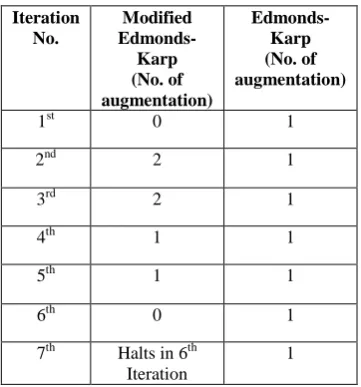
The following table shows the comparison between two algorithms and also shows the above fact.
Table 3. Iteration – augmentation relationship
Iteration No.
Modified Edmonds-Karp (No. of augmentation)
Edmonds-Karp (No. of augmentation)
1st 0 1
2nd 2 1
3rd 2 1
4th 1 1
5th 1 1
6th 0 1
7th Halts in 6th
Iteration
1
As the table shows, the modified algorithm calculates the maximum flow after 6 augmentations with 6 iterations while the Edmonds-Karp algorithm calculates the maximum flow after 7 augmentations with 7 iterations. Thus, it can be seen that for such a graph with less vertices also, the modified algorithm takes 1 less iteration than the Edmonds-Karp algorithm. And if the no. of vertices in the graph is much larger, then the modified algorithm will perform extremely better than the Edmonds-Karp algorithm. The Edmonds-Karp algorithm runs in O (𝐄𝟐𝐕) while the modified algorithm runs in O (𝐄𝟐 𝐥𝐨𝐠𝟐𝐂) where C is maximum edge capacity in the
graph. Hence it can be said that the modified algorithm will perform better than Edmonds-Karp algorithm for any graph where V > 𝐥𝐨𝐠𝟐𝐂and this condition generally holds for most graphs and if no. of vertex (V) is more, then obviously no. of edges (E) will be more.
The following table shows some cases of graph where it can be seen that even though the difference between V and
[image:5.595.77.258.264.458.2]𝐥𝐨𝐠𝟐𝐂 is less, the difference between 𝐄𝟐 𝐥𝐨𝐠𝟐𝐂 and 𝐄𝟐𝐕 considerably larger because of 𝐄𝟐.
Table 4. Comparison of complexities of two algorithms
No. of vertices
V
No. of edges
E
Maximum capacity
C
𝐥𝐨𝐠𝟐𝐂 𝐄𝟐 𝐥𝐨𝐠𝟐𝐂 𝐄𝟐𝐕
15 25 128 7 4375 9375
10 18 75 6.229 2018 3240
12 20 30 4.907 1963 4800
15 23 32 5 2645 7935
5.
RESULTS
The modified Edmonds-Karp algorithm returns a maximum flow
This algorithm uses the Ford-Fulkerson method. It repeatedly augments the flow along an augmenting path until there are no augmenting paths of capacity greater ≥ 1. Since all the capacities are integers, and the capacity of an augmenting path is positive, this means that there are no augmenting paths whatsoever in the residual graph. Thus, by the max-flow min-cut theorem,the modified Edmonds-Karp algorithm returns a maximum flow.
For a given number I, an augmenting path of capacity at least I can be found in O(E)time, if such a path exists.
The capacity of an augmenting path is the minimum capacity of any edge on the path, so we are looking for an augmenting path whose edges all have capacity at least K. Do a breadth-first search or depth-breadth-first-search as usual to find the path, considering only edges with residual capacity at least K. (Treat lower-capacity edges as though they don.t exist.) This search takes O(V + E) = O(E) time.(Note that |V| = O(E) in a flow network.)
The new modified Edmonds-Karp algorithm runs in O (𝐄𝟐 𝐥𝐨𝐠𝟐𝐂).The time complexity is dependent on the loop of steps 6-12 because the steps 1-5 take O (E) time. The outer while loop executes O ( 𝑙𝑜𝑔2𝐶) times, since I is initially O(C) and is halved on each iteration, until K < 1. The inner while loop executes O (E) times for each value of I and as shown in above result each iteration takes O(E) time. Thus, the total time is O(𝐸2 𝑙𝑜𝑔2𝐶).
6.
CONCLUSION AND FUTURE SCOPE
The basic classical techniques used in maximum-flow algorithms can be adapted to solve other network-flow problems. By solving maximum flow problem we can consider a class of similar problems that seek to maximize the flow through a flow network while at the same time minimizing the cost of that flow. So it can be concluded that computing the Maximum Flow in the flow network graph produces a maximal matching set for the original Bipartite Matching problem. And on further reflections, it can be used to solve the more powerful Minimal Cost Flow problem, which enables us to immediately solve the Transshipment, Transportation, and Assignment problems.
The modified Edmonds-Karp algorithm returns a maximum flow and this algorithm takes less no. of iterations and less
augmentation to calculate the maximum flow. An
algorithm runs in O(E2 log2C) while Edmonds-Karp algorithm runs in O (E2V). So, finally it can be concluded that the modified Edmonds-Karp algorithm performs better in most cases compared to Edmonds-Karp algorithm. The Ford Fulkerson algorithm is the general algorithm to solve the network flow problems and its improvement is Edmonds-Karp algorithm which performs better than it. So, In future more optimized algorithms can be developed to solve the network flow problems in more efficient manner.
7.
REFERENCES
[1] Andrew V. Goldberg, Eva Tardos and Robert E. Tarjan
(1988). A new approach to the maximum-flow problem. Journal of the ACM. 35:921–940
[2] Jack Edmonds and Richard M. Karp (1972). "Theoretical improvements in algorithmic efficiency for network flow problems". Journal of the ACM 19 (2): 248–264. doi:10.1145/321694.321699
[3] Bazarra, M. and J. Jarvis. Linear Programming and Network Flows. John Wiley & Sons, 1977.
[4] Ford, L. R. Jr. and D. R. Fulkerson. Flows in Networks. Princeton University Press, 1962.
[5] “Maximum Flow Problem”
http://en.wikipedia.org/wiki/Maximum_flow_problem
[6] “Recent Developments in Maximum Flow Algorithms”
www.springerlink.com/index/tfdyr7n9xyer80p7.pdf
[7] Ravindra K. Ahuja and James B. Orlin. “A fast and simple algorithm for the maximum flow problem”. Operations Research, 37(5):748–759, 1989.
[8] Ravindra K. Ahuja, James B. Orlin, and Robert E. Tarjan. “Improved time bounds for the maximum flow problem”. SIAM Journal on Computing, 18(5):939–954, 1989.
[9] “Network Flow Programming”
www.sce.carleton.ca/faculty/chinneck/po/Chapter10.pdf.
[10] Mircea Parpalea. Min-Max Algorithm For ThParametric Flow Problem Bulletin of the Transilvania University of Bra¸sov , Vol 3(52) , 2010