An Application of Genetic Algorithm for Solving Academic Personnel Planning Problems in University Management System via Fuzzy Goal Programming with Penalty Functions

(1)

An Application of Genetic Algorithm for Solving

Academic Personnel Planning Problems in University

Management System via Fuzzy Goal Programming with

Penalty Functions

Debjani Chakraborti

Department of Mathematics

Narula Institute of Technology

Kolkata, West Bengal, India

Papun Biswas

Department of Electrical Engineering,

JIS College of Engineering

Kalyani-, West Bengal, India

ABSTRACT

This article demonstrates how the genetic algorithm (GA) approach can efficiently be used to the penalty function based fuzzy goal programming (FGP) formulation for modelling and solving academic resource planning problems in University management system.

A demonstrative case example of the University of Kalyani, West Bengal (W.B), India is considered to expound the potential use of the approach. The proposed model is compared with the conventional FGP solution of the problem.

Keywords

Fuzzy programming, Goal programming, Fuzzy goal programming, Genetic algorithm, Penalty function.

1. INTRODUCTION

The increase of social awareness for betterment of social life as well as uplift in technological aspects has created a deep interest in higher education to the new study areas in the current technological affluent society in the recent years from the view points of widening the academic interest as well as opening the scope of employment to different emerging activity areas.

As a matter of fact, worldwide initiative for opening of new academic departments in university system has been taken in the past few years by most of the higher academic institutions. It is to be mentioned here that in most of the developed countries, tuition fees play the major roles to meet the economic constraints of running the academic organizations. But, in case of a developing country like India, universities are mainly run by the national income of a Government. Again, since the Universities are not the profit making organizations, opening of a new academic unit means increase of financial load to a University within the limited allocation of budget in a financial year.

In such a case, proper planning for academic staff allocation and setting of other assisting personnel within the existing infrastructure is inevitably needed for sustainable growth of the new units in the decision making horizon.

From a historical perspective, early works on education planning were studied by Gani [1] in 1963 and Platt [2] in 1962 as the applications of quantitative methods in the area of management science. During 1960s, studies on planning, programming and budgeting system in higher education were taken place rapidly and circulated widely in the literature. The

survey of works in the field of higher education was conducted by Rath [3] and Hufner [4] in 1968. Different management science models to academic resource planning for enrichment of higher education were investigated [5, 6].

A comprehensive bibliography on the state-of-the-art of modelling aspects of academic planning for improvement of the quality of education studied from 1960s to early ’70s was first prepared by Schroeder [7] in 1973. Thereafter, worldwide efforts for implementation of management science models to enrich the various activities of academic institutions were taken place from the view point of potential growth of socio-economic conditions of a nation.

Now, since most of the academic planning problems are multiobjective in nature, goal programming (GP) approach [8, 9] as one of the most promising and flexible tool for multiobjective decision analysis has been successfully implemented to university management system by Schroeder [10], Walters et al. [11], Franz et al. [12], and others. The extensive study on academic planning has been further surveyed by White [13] in 1987. The several other modelling aspects for different higher academic planning problems have also been studied by Pal and Basu [14] in 1997 and Kwak and Lee [15] in 1998.

Now, in a real-life decision situation, it is to be observed that the decision maker (DM) is often faced with the problem of setting precise parameter values to the decision problems due to inherent imprecise in nature of them as well as ambiguity in human judgments. In such a situation, crisp mathematical programming approaches fail to produce proper solutions in practical decision situations.

To overcome the above difficulty, FGP approach [16,17] in the field of fuzzy programming (FP) [18,19] and interval goal programming (IGP) [20] in the area of interval programming (IvP) [21] as the extension of conventional GP has been developed for solving multiobjective decision problems in imprecise (inexact) decision environment. The FGP as well as IGP approaches to university planning problems and other decision problems have been studied by Pal et al. [22, 23] in the past.

(2)

The above difficulty may also arise due to inexactness of the expert’s knowledge about the parameter values as well as setting of highly optimistic target levels of achieving the objectives. As a matter of fact, decision trouble is frequently encountered in solving practical decision problems.

Now, for managerial decision making, the problem of achieving goal values in different ranges instead of attaining the assigned target levels of the goals as in conventional GP formulation, the concept of penalty functions with the incorporation of marginal penalties for minimizing the deviations for goal achievement in different ranges has been well discussed by Romero [24] in 1991.The concept has been further extended by the active researchers [25, 26, 27, 28, 29, 30] in the past for solving IGP problems.

The penalty function approach to the GP model of an academic planning problem have also been studied by Pal et al. [14] in the past.

In the decision making environment, GAs based on natural selection and population genetics, initially introduced by Holland [31], have also appeared as robust computational tools in the field of optimization problems. The use of GAs on the framework of multiobjective decision making (MODM) problems have been investigated by the pioneer researchers in the field and implemented to practical problems. But exploration of the potential use of GAs to real-life MODM problems (crisp or fuzzy) is at an early stage.

The GA method [31, 32] as the direct random search approach to university management problems have been studied by Wang [33] and Mozos et al. [34] in the past. The use of GA scheme to university management has also been studied by Pal et al. [35] in the past. However, the use of GA to penalty function based FGP formulation of MODM problems is yet to be documented in the literature.

In the proposed approach, requirement of total full-time teaching staff and allocation of pay-roll budget to each of academic departments are fuzzily described. The recruitment of minimum number of teaching and non-teaching staff and maintaining of certain ratios of part-time teaching staff and non-teaching staff individually with full-time teaching staff, and a ratio of total number of students with total teaching staff in each department for smooth functioning of the academic activities of the departments are considered as constraints in the academic planning horizon.

In the model formulation of the problem, the concept of penalty functions for measuring the degree of achievement of membership goals in different ranges for the defined fuzzy goals and thereby arriving at a satisfactory decision is considered. The percentage achievements of goals in different ranges are defined first in terms of achievement of the membership values to the extent possible by minimizing the associated deviational variables in the goal achievement function.

In the solution process, an GA scheme is iteratively used to solve the problem for achievement of the defined goals on the basis of the priorities assigned to them without linearizing the defined fractional constraints, unlike the classical approaches, in the decision making environment.

A case example of the University of Kalyani, W.B, India is considered to illustrate the proposed model. The model solution is compared with the existing staff allocation pattern as well as the conventional Minsum FGP solution approach in the decision making environment.

Now, the general FGP problem formulation is presented in the following Section 2.

2. PROBLEM FORMULATION

The generic form of a multiobjective FP problem can be presented as:

Find

X

(x

1

,

x

2

,...,

x

n

)

so as to

satisfy Z_k(X) b_k

~

 

 

 

 





, k =1,2,...,K (1)

subject to

    

  

         



 



m

n_|_AX _b,_X _0,_b _R

R X S

X (2)

where X is the vector of decision variables,

~



and indicate

the fuzziness of ≥ and ≤ restrictions, respectively, in the sense of Zimmermann [36], and where bk is the imprecise aspiration

level of the k-th objective Zk (X), (k = 1,2,..., K), A is the

technological coefficient matrix, b is the vector of right-hand side values. It is assumed that the feasible region S (≠Φ) is bounded.

Now, in a fuzzy decision making situation, the fuzzy goals are to be characterized by their respective membership functions.

2.1 Characterization of Membership

Function

Let

t

_l_k and tuk be the lower- and upper-tolerance ranges,

respectively, for achievement of the aspired level bk of a k-th

fuzzy goal. Then, the membership function, say

μ

_k(X), for the fuzzy goal Zk(X) can be characterized as follows [17].

For

~



type of restriction,

μ

k(X) takes the form:

      

 

   







, t b (X) Z if , 0

, b (X) Z t b if , t

) t (b (X) Z

, b (X) Z if , 1

(X) μ

k k k

k k k k k

k k k

k k

k

l l

(3) where (bk -

t

lk) represents the lower-tolerance limit for achievement of the stated fuzzy goal.

Again, for type of restriction,

μ

_k(X) becomes

      

 

   







, t b (X) Z if , 0

, t b (X) Z b if , t

(X) Z ) t (b

, b (X) Z if , 1

(X) μ

uk k k

uk k k k uk

k uk k

k k

k

(4) where (bk + tuk) represents the upper-tolerance limit for

achievement of the stated fuzzy goal. Then, the FGP formulation for the defined membership functions are presented in the Section 2.2.

2.2 FGP Model Formulation

In FGP model formulation, the membership functions are transformed into membership goals by assigning the highest degree (unity) as the aspiration level and introducing under- and over-deviational variables to each of them. Then, in the goal achievement function, the under-deviational variables

~



~

(3)

are minimized on the basis of the importance of achieving the aspired goal levels in the decision making context.

Now, since multiple goals are involved with the problem and they often conflict each other for achievement of their aspired goal levels, a priority based FGP model for goal achievement is considered in the decision making situation.

The FGP model of the problem for the defined membership functions under a pre-emptive priority structure appears as Find

X

(x

₁

,

x

₂

,...,

x

_n

)

so as to

Minimize Z[P₁(d),P₂(d),...,P_h(d),...,P_H(d)]

and satisfy d d 1,

t ) t (b (X) Z

k k k

k k

k     

 

, 1 d d t

(X) Z ) t (b

k k uk

k uk

k  _ _ _

, 0 d , dk k

 

k = 1, 2,..., K,

(5) where, Ph (d–) represents the vector of H priority achievement

function, and dk,dk are the under- and over-deviational

variables of the k-th goal. Ph (d–) is a linear function of the

weighted under-deviational variables, where Ph (d –

) is of the form:

Ph (d

–

) = Kw d ; ,

1

k hk hk

 



 _{h = 1, 2,..., H; (H}__{K), (6)}

where

d

_hk is renamed for d_k to represent it at the h-th priority level,

w

_hk (>0) is the numerical weight associated with

d

_hk and it designates the weight of importance of achieving the aspired level of the k-th goal relative to other which are grouped at the h-th priority level and where

w

_hk

values are determined as [17]:

(4) in (X) μ defined for the ,

(3) in (X) μ defined for the , w

k )

(t 1

k )

(t 1

hk

h u k

h k

    

 l

(7) where,

(t

l_k

)

_h and

(t

uk

)

hare used to present

t

lk and

t

uk,

respectively, at the h-th priority level.

It is worthy to mention here that the notion of pre-emptive priorities of the goals actually hold on the concept that the h-th priority Ph is preferred to the next priority Ph + 1 regardless

of any multiplier associated with Ph + 1, h= 1,2,…, H.

Also, the relationship among the priorities is: P1 >>> P2 >>> . . . >>> Ph >>> . . . >>> PH ,

which implies that the goals at the highest priority level (P1)

are achieved to the extent possible before the set of goals at the second priority level (P2) is considered, and so forth.

Now, an GA scheme for solving the problem (5) is presented in the following Section 3.

3. DESCRIPTION OF GA SCHEME

Now, in the literature of GAs, there is a large number of schemes [31, 32] for generating new populations with the use of different operators: selection, crossover and mutation. However, the basic steps of the GA procedure with the core functions adopted in the solution process are presented via the following steps.

Step1. Representation and Initialization

Let M denote the binary coded representation of a chromosome in a population as M = {g1, g2,..., gn}. The

population size is defined by pop_size, and pop_size chromosomes are randomly initialized in its search domain.

Step2

.

Fitness Function

The fitness value of each chromosome is judged by the value of the goal achievement function defined with the priorities of the goals. The fitness function is defined as

eval (M

v

) = (Z

h

)

v

=

v K

1 k

hk hk

d

w



















  

,

where (Z

h

)

v

represents the h-th priority factor of the

goal achievement of the function

Z

and the subscript

‘

v

’ refers to the fitness value of the selected

v

-th

chromosome,

v

= 1, 2, ..., pop_size. The best

chromosome with largest fitness value at each

generation is determined as

M* = min {eval(Mv) | v = 1, 2, ..., pop_size}, depending

on searching of the best value of an objective.

Step3. Selection

The simple roulette-wheel scheme [32] is used for selecting two parents for mating purposes in the genetic search process.

Step4. Crossover

The parameter pc is defined as the probability of crossover.

The arithmetic crossover (single-point crossover) operation of a genetic system is applied here in the sense that the resulting offspring appear with very close characteristics of parents and always satisfy the linear constraints set S ( ). Here, a chromosome is selected as a parent for a defined random number r  [0, 1], if r < pc is satisfied. Again, in the

reproduction process, the arithmetic crossover for two selected parents M1, M2 can be defined as

G1 = 1M1 + 2M2 and G2 = 2M1 + 1 M2

for producing two offspring G1 and G2 (G1 and G2



S

)

where ₁ , ₂  0 with ₁+₂= 1.

Step5. Mutation

As in the conventional GA scheme, a parameter pm of the

genetic system is defined as the probability of mutation. The mutation operation is performed on a bit-by-bit basis, where for a random number r  [0, 1], a chromosome is selected for mutation provided that r < pm.

Step6.

Termination

The execution of the whole process terminates when the

fittest chromosome is reported at a certain generation

number in the solution search process.

Remark: Since GAs are satisficers rather than optimizers [31], in the process of using the GA method to the problem, the system constraints are also made flexible by introducing under- and over-deviational variables to each of them in the notion of searching the most satisfactory solution in the expanded flexible region S in goal satisficing philosophy of conventional GP [8,9]. The system constraints are then termed as the flexible goals.

The flexible goals in explicit form can be presented as:

a

ij

x

j



d

i



d

= pay-roll budget allocation to the department i at time period t.

(ii) Definition of decision variables:

The following decision variables are involved in the proposed model.

ij t

f

= number of FTS in the department i, rank j at the time period t.

it

n

= number of NTS in the department i at the time period t.

it

p

= number of PTS employed in the department i at the time period t.

Now, the fuzzy goals and constraints of the problem are described in the following Section 4.

4.1 Description of Fuzzy Goal and

Constraints

4.1.1 Fuzzy goal description

Two types of fuzzy goals are involved with the problem. They are described as:

(i) FTS goals:

For potential academic performance of the departments, an estimated number of total FTS should always be employed to each of the departments by the University management. But, due to limitation of budget, requirement of FTS to an aspired level is fuzzy in nature at a planning period t.

The fuzzy goal expressions appear as





J

1 j

ijt

f

~



[FTS]

it, i=1, 2,…,I. (8) Now, in conventional framework of GP with penalty

functions, the goals are normalized to make the goals commensurable as well as to measure the goal achievement in terms of percentage.

Then, the goal expression in (8) takes the form

_ijt

J

1

j it

f

[FTS]

100 















~



100, i = 1, 2,…, I (9)

(ii) Budget goal:

Due to limitation of total available budget to run the University, the pay-roll budget for each department is fuzzily described.

The budget goal expression appears as:



  



 

J

1 j

it it I

1 i it it I

1 i ijt ijt I

1 i

p [P ] n

[NS] f

[TS]

[B] it

(10)

Then, in percentage scale, the expression in (10) takes the form:



  



 

J

1 j

it it it I

1 i it it it I

1 i ijt ijt it I

1 i

.p )[P] [B]

100 ( .n )[NS] [B]

100 ( .f )[TS] [B]

100 (

100 (11)

Then, the membership function representations of the stated goals and measuring of the achievement grades of membership functions for incorporation of penalty functions are presented via a case example provided in the Section 5. Now, the constraints of the problem are defined as follows:

4.1.2 Crisp constraint description

The two types of crisp constraints (linear and fractional) are involved with the staff allocation structure of the problem.

(i) FTS Constraints:

To run the academic curriculum, a minimum number of FTS at each rank need have to be provided in each of the departments.

The FTS constraints appear as:

fijt[F]ijt, i1,2,...,I; j1,2,...,J (12)

(ii) NTS constraints:

To perform the official and teaching related activities, a minimum number of NTS should be employed to each of the departments.

The NTS constraints appear as:

nit[N]it, i1,2,...,I; (13)

(iii) PTS-FTS ratio constraint:

When the FTS can not be employed at a time period t, PTS at a certain ratio to FTS should be provided in each of the departments.

~



~

(5)

Salary in Percentage

39%

31% 22%

6% 2%

Professor Asc. Professor Ast. Professor PTS NTS The ratio constraints in fractional form can be presented as:

_J i

1 j

ijt it _[r]

f

p _





, i=1,2,…,I. (14)

(iv) ST-TTS ratio constraint

For smoothing the academic activities, a certain ratio of ST and TTS should be maintained in each of the departments.

The constraints take the form:

[s]

,

i

1,2,...,

I

)

p

f

(

[S]

i J

1 j

it ijt

it

_







(15)

(v) NTS-TTS ratio constraints

To meet the need of assisting the academic and official activities, a certain ratio of NTS and TTS should be provided to each of the departments.

The ratio constraints can be expressed as:

_J i

1 j

it ijt

it

[R] ) p (f (

n

 





, i = 1, 2, …, I (16)

Now, the executable FGP model formulation of the problem by grafting penalty functions and thereby solving the problem is presented through a demonstrative case example in the Section 5.

5. AN ILLUSTRATIVE EXAMPLE: A

CASE STUDY

The academic resource allocation problem of the University of Kalyani, West Bengal, India is considered to demonstrate the application potential of the proposed approach. To illustrate the potential use of the approach, the staff allocation problem of the four new departments: Physiology (PH), Molecular Biology and Bio-Technology (MB-BT), Microbiology (MB) and Geography (GEO) under the faculty of science, University of Kalyani, INDIA is taken into account. The required data for the proposed model was according to the revision of pay scale under 6th_pay

commission on the basis of the memorandum of the Principal Secretary, Higher Education Department, Bikash Bhavan, Kolkata bearing No. 715 –Edn (U) dated 18.12.2009 for the financial year 2009–2010.

[image:5.595.311.548.82.215.2]

The decision variables and different types of data involved with the problem are summarized in the Tables 1-3.

Table 1.Data Description of Fuzzy Goal Levels of FTS

Department PH (1) MB-BT

(2) MB (3) GEO (4)

FTS 6 6 6 8

Table 2.Annual Average Salary for FTS, NTS and Remuneration for PTS

Rank Salary (Rs.) Remuneration (Rs.)

Professor 9.17 Lac -

Associate

Professor 7.2 Lac -

Assistant

Professor 5.16 Lac -

PTS(Guest

Professor) 1.5 Lac -

NTS - 0. 5 Lac

The total Pay-roll Budget 293.26 Lac.

The Pie Chart of Budget distribution (in percentage) for salary of staff is presented in the Figure 1.

Fig 1: Budget distribution of salary of staff Then the data for the ST, the ratios of PTS-FTS, TTS-ST, NTS-TTS and are given in Table 3.

Table 3.Data Description of ST and the Ratios of PTS-FTS, TTS-ST, NTS-TTS

[image:5.595.311.553.259.375.2]

The bar diagram of the number of students in different departments is shown in the following Figure 2.

Fig 2: Graphical Representation of number of students in different departments.

Department Number of Students

PTS -FTS

TTS - ST

NTS – TTS

PH 30 1:4 1:7 2:5

MB&BT 24 1:4 1:7 2:5

MB 32 1:4 1:7 2:5

[image:5.595.313.548.578.677.2]

(6)

Now using the data tables and the other necessary collected data, construction of the fuzzy goals and the crisp goals are described in the Section 5.1.

Here, since the variables are introduced with running period (t = 1), the time specification (t) is omitted for simplicity during the presentation of the case model.

5.1 FTS Goals

In the fuzzy decision making situation, it is assumed that 80% achievement is the lower tolerance limit as desired by the DM for all the defined FTS goals of the four departments.

Then, following the expressions in (9), the membership goals are obtained as:



16.67(f f f ) 80



d d 1 0.05 11 12 13   1 1 

 

(PH department) (17)



16.67(f f f ) 80



d d 1

05 .

0 ₂₁ ₂₂ ₂₃   ₂ ₂

(MB-BT department) (18)



16.67(f f f ) 80



d d 1

05 .

0 31 32 33   3 3

 

(MB department) (19)



12.5(f f f ) 80



d d 1

05 .

0 ₄₁ ₄₂ ₄₃   ₄ ₄ 

(GEO department) (20) Now, in the conventional FGP approach, achievement of the

highest membership value (unity) by minimizing the under-deviational variables di(i1,2,3,4)



to the extent possible is

considered, where any di (0)



indicates the measure of non-achievement of an aspired membership value.

But, in a practical decision situation, it is to be observed that achievement of fuzzy objectives in different intervals are to be taken into account [37,38] instead of taking them singled valued as employed in the conventional FGP approach to decision problems. Actually, consideration of this situation arises due to inexactness of the environment of making decision.

To overcome the above situation, relaxation of tolerance ranges of fuzzy goals for their achievement in different intervals up to certain defined goal level for each of them can be considered, and the grafting of penalty functions for measuring the actual degree of achievement of a fuzzy goal can be taken into account.

The inclusion of penalty functions to the formulated model by defining penalty scales is presented as follows:

Grafting of Penalty Functions

In the conventional GP approach, the penalty functions are defined by the deviational variables associated with the achievement of goal values in the different ranges, and they are minimized in the goal achievement function on basis of the introduced marginal penalties [39] where marginal penalties indicate the relative weights of importance of achieving the goals by minimizing the associated deviational variables.

In the present decision situation, the deviational variables are expressed in terms of under-achievement of the defined membership values for goal achievement in different specified ranges.

Now, for the defined membership goals in (5), it is to be followed that achievement of highest membership value of a goal is made by minimizing the under-deviational variables. Here, above 100% achievement of a fuzzy goal means that the attainment of a membership value is more than unity. In such

a situation the marginal penalty is assigned as zero and the DM is overly satisfied here. The other penalty scales for grafting the penalty functions for goal attainment of all the defined FTS goals of the departments are considered the same.

The penalty scale representations to evaluate (17), (18), (19), (20) are summarized in the Table 4.

Table 4. Penalty Scales for FTS Goals Goal

attainment range (in %)

Under-deviation

(in %)

(AMV,Under-

deviation) MP

Over 100 0 (above unity, 0) 0

_i_l for each of the defined ranges, the penalty function goals in the form of conventional goals can be presented as:

0.2 η η

d_i1 _i1 _i1  (25)

1 . 0

d_i₂_i₂_i₂ (26)

2 , 1 , 4 , 3 , 2 , 1 i , 0 , i

i    

 

l

l l

Now, to make a control of keeping goal achievement within a specified range, d_i_land_i_l,i1,2,3,4,l1,2are to be

minimized in the goal achievement function of the executable FGP model of the problem. Again involvement of i2(0)



in the solution indicates further relaxation for goal achievement within an interval.

Here, since below 70% achievement is not acceptable, it can reasonably be assumed that

4 , 3 , 2 , 1 i , 1 . 0

2

i  



(7)

5.2 Budget Goal

From the fuzzy goal description of budget goal in (11), the upper tolerance ranges for budget allocation are involved in the decision situation. It is assumed that 15% more allocation as relaxation of the budget limit is introduced by the DM.

Then, using the prescribed data and following the expression in (5), the membership goal of the fuzzy budget goal in (11) can be obtained as:

1 d d )}] p p p p ( 51 . 0 ) n n n n ( 17 . 0 ) f f f f ( 75 . 1 ) f f f f ( 44 . 2 ) f f f f ( 12 . 3 { 115 [ 07 . 0 5 5 4 3 2 1 4 3 2 1 43 33 23 13 42 32 22 12 41 31 21 11                          (28) Now, it is to be followed from the expression in (28) that any

over-achievement from 100% of the defined fuzzy goal level is represented by the under-deviation from the highest membership value. Again, for any goal value lower than 100%, the fuzzy goal is overly satisfied which is indicated by the value of the over-deviational variable d and for which 5

attainment of membership value is found to be more than the aspired level (unity). As a matter of fact, similar to the case of membership goal achievement for FTS goals, d is to be 5

minimized here in the goal achievement function, which is not alike the conventional GP with penalty functions where over-deviational variable of a goal is minimized for goal achievement in a given interval.

[image:7.595.315.543.426.652.2] [image:7.595.49.287.432.533.2]

Now, in the decision situation, consideration of different goal achievement ranges and penalty scale representations of them in terms of membership goal deviations is summarized in the Table 5.

Table 5. Penalty Scales for Budget Goals Goal attainment range (in %) Under-deviation (in %) (AMV,Under- deviation) MP

Below100 0 (above unity, 0) 0 100-115 15 (1, 0.15)

0.066 115-125 10 (0.9, 0.1) 0.1 Above 125  



Note: The meaning of the abbreviations is the same as defined in the Table 4. Now, for the defined penalty scales in the Table 5, grafting of the penalty functions for achievement of budget goal can be described in an analogous way to the case of goal achievement for FTS goals presented in the Section 5.1.

The membership goal in (28) with penalty functions can be presented as 1 d d )}] p p p p ( 51 . 0 ) n n n n ( 17 . 0 ) f f f f ( 75 . 1 ) f f f f ( 44 . 2 ) f f f f ( 12 . 3 { 115 [ 07 . 0 5 4 3 5 4 3 2 1 4 3 2 1 43 33 23 13 42 32 22 12 41 31 21 11                            l l

(29) (12.29)

15 . 0 d535353

 

 ₍₃₀₎

1 . 0

d₅₄ ₅₄ ₅₄  (31)

Then, the deviational variables to be minimized in the achievement function are d and 5l 5(0)



l , l = 3, 4.

Again, since over-deviation of the budget goal is restricted to 25%, similar to the case of achievement of an FTS goal,

1 . 0

5 



4 (32) is introduced as a constraint in the formulated model.

Now, the system constraints of the model are described in the Section 5.3.

5.3 Description of System Constraints

(a) FTS constraints

On the basis of the current work loads of the departments, a minimum number of FTS at each rank need to be employed to each of the departments. The FTS constraints appear as:

1 11

f , f₁₂1, f₁₃2, 1

21

f , f₂₂1, f₂₃2, 1

31

f , f₃₂2, f₃₃2, 1

41

f , f₄₂3, f₄₃1.

(33)

(b) NTS constraints

The constraints can be presented as: 2 n 2, n 2, n 2,

n₁ ₂ ₃ ₄

(34) (c) Ratio constraints

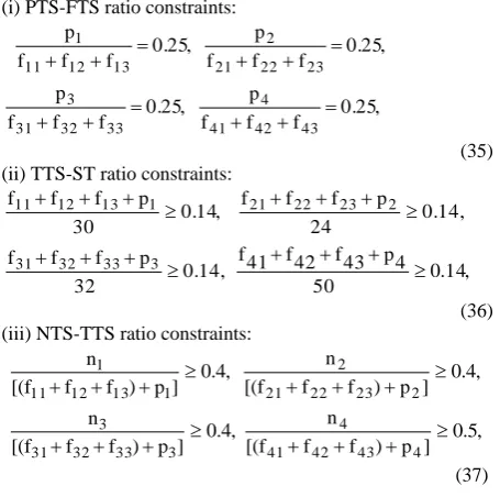
Using the data in the Table 3, the different ratio constraints are obtained as follows:

(i) PTS-FTS ratio constraints:

f f f 0.25, p 13 12 11 1 _ 

 f f f 0.25,

p 23 22 21 2 _   , 25 0. f f f p 33 32 31 3 _ 

 f f f 0.25,

p 43 42 41 4 _   (35) (ii) TTS-ST ratio constraints:

, 14 0. 30 p f f

f₁₁ ₁₂ ₁₃ ₁

    ₂₄ 0.14, p f f

f₂₁ ₂₂ ₂₃ ₂

    0.14, 32 p f f

f31 32 33 3 _

, 14 . 0 50 4 p 43 f 42 f 41 f     (36) (iii) NTS-TTS ratio constraints:

, 4 . 0 ] p ) f f [(f n 1 13 12 11 1 _  

 [(f f f ) p ] 0.4,

n 2 23 22 21 2 _    , 4 . 0 ] p ) f f [(f n 3 33 32 31 3 _  

 [(f f f ) p ] 0.5,

n 4 43 42 41 4 _    (37) (12.37) Now, for the defined goals and constraints, formulation of the

executable model as an extension of the FGP model in (5) is presented in the following Section 5.4.

(8)

5.4 Executable FGP Model Formulation

The two priority factors are introduced for achievement of the model goals in the decision making context.

The first priority (P1) is assigned to the goals with highest

membership value and the second one (P2) is assigned to the

defined penalty function goals.

The executable model under the framework of priority based FGP with penalty functions appears as

Find (fij,pi,ni | i=1,2,3,4; j=1,2,3) so as to

Minimize Z =

}, d 1 . 0 d 066 . 0

) d d d d ( 1 . 0 ) d d d d ( 05 . 0 { P [

54 53

42 32 22 12 41

31 21 11 1

 

    

  

 

      

}], 1 . 0 066 . 0

) (

1 . 0 ) (

05 . 0 { P

54 53

42 32 22 12 41

31 21 11 2

 

    

  

   

              

and satisfy the goal expressions in (21)-(27), (29)-(32) subject to the constraints in (33)-(37).

The proposed GA approach is used to solve the problem. Here, the goal achievement function (Z) represents the evaluation function in the genetic search process for achieving the goals on the basis of the assigned priorities.

The programming language C is used in the process of coding the evaluation program. The environment of execution is Intel Pentium IV with 2.66 GHz. Clock-pulse and 1 GB RAM. The, chromosome length = 30 is considered with a view to searching solution in the domain of feasible solution set (S) defined in the decision situation. The population size as in the standard GA method is taken 100. The number of generations = 300 is initially taken to conduct the experiment.

The different experiments with the different values of pc (0 <

pc <1) and pm(0 < pm <1), in the ranges (0.7 < pm < 0.9) and

(0.03 < pm < 0.8) are made in the proposed GA scheme. It is

found that pc = 0.8 and pm = 0.08 are successful in the

decision search process.

The resulting model solution is presented in the Table 6.

Table 6. Solution for Staff Allocation under the proposed Model

Department PH MB-BT MB GEO Professor

Associate Professor Assistant Professor PTS (Guest Prof.) NTS

2 2 3 2 2

2 3 2 4 5

4 2 4 4 4

5 3 3 2 5

The data of the existing staff structure of the departments are presented in the Table 7.

Table 7. Existing Staff Allocation Structure (2009-2010) Department PH MB-BT MB GEO Professor

0 1 1 3 8

0 0 2 2 35

0 1 1 2 8

0 1 1 5 7

A comparison of the model solution with the existing staff allocation displayed in the Table 7 shows that a satisfactory solution is achieved under the proposed model in the decision making environment.

Note: If the defined penalty functions are not taken under consideration and achievement of the defined membership goals in (17)-(20) and (28) are only taken into account in minisum FGP formulation of the problem and if all the goals are treated at the same priority level, then the obtained solution of the problem is presented in the Table 8.

Table8. Model Solution under the Minsum FGP Approach

Department PH MB-BT MB GEO Professor

1 1 6 2 7

2 2 4 2 4

2 3 3 2 4

1 3 4 2 7

The following Figure shows a comparison of the solutions obtained by the three different cases.

Fig 3: Comparison of the solutions of the approaches A further comparison of the model solution with the solution in the Table 8 shows that the proposed approach is a superior one from the view point of achieving the desired staff levels for smooth functioning of the academic activities of the departments.

6. CONCLUSION

The main advantage of using the proposed GA approach is that the computational load involved with the traditional approaches for linearization of the real-life problems with fractional criteria can be avoided here in the solution process. Moreover, the most satisfactory decision can easily be reached here in the solution search process of the proposed GA method without involving extra computational burden with redefining the model as involved in the decision process of using the traditional approaches.

Further, the FGP with penalty function approach to academic personnel planning problem in a University system demonstrated in the paper provides a new look into the way of analyzing the achievement of the fuzzily described objective goal levels in different intervals on the basis of needs and desires of the departments towards enrichment of academic activities of a university. The main advantage of using the proposed approach is that the grafting of penalty functions makes the model a flexible one to reach a satisfactory decision in the academic planning horizon.

(9)

parameter values involved in both the objectives and constraints in the decision making environment. The IGP with penalty function method to university planning in inexact decision environment may be a problem for future study.

Finally, it is expected that the modelling aspects of the academic planning problem presented here can contribute to future research of different real-life problems for managerial decision making.

7. ACKNOWLEDGMENTS

The authors are thankful to the anonymous Reviewers of IJCA for their valuable comments and suggestions which have led to improve the quality and clarity of presentation of the paper.

8. REFERENCES

[1] Gani, J. 1963 Formulae of Projecting Enrollments and Degrees Awarded in Universities, Journal of Royal Statistical Society, Vol. 126, No. 3, 400-409.

[2] Platt, W.J. 1962 Education-Rich Problems and Poor Markets, Management Science, Vol. 8, No. 4, 408-418.

[3] Rath, G.I. 1968 Management Science in University Operation, Management Science, Vol. 14, No. 8, B-373-384.

[4] Hufner, K. 1968 Economics of Higher Education and Educational Planning-A Bibliography, Socio-Economic Planning Sciences, Vol. 2, No. 1, 25-101.

[5] Richard, W.J. and Levine J. 1965 A new Tool for Education Administrators, Report to the Commission on the Financing of Higher Education,University of Toronto Press, Toronto, Ontario, Canada.

[6] Williams, H. 1966 Planning for Effective Resource Allocations in Universities, American council on Education, Washington, D.C.

[7] Schroeder, R.G. 1973 A survey of Management science in University operations, Management Science, Vol. 19, No. 8, 895-906.

[8] Ignizio, J. P. 1976 Goal Programming and Extensions. Lexington Books. Lexington MA.

[9] Romero, C. 1986 A Survey of Generalized Goal Programming (1970-1982), European Journal of Operational Research, Vol. 25, No. 2, 183 – 191.

[10] Schroeder, R.G. 1974 Resource Planning in University Management by Goal Programming, Operations Research, Vol. 22, 700 – 710,

.

[11] Walters, A. J., Mangold, J. and Haran, E. G. P. 1976 A Comprehensive Planning Model for Long-Range Academic Strategies, Management Science, Vol. 22, No. 7, 727 – 738.

[12] Franz, L. S., Lee, W. M. and Van Horn J. C. 1981 An Adaptive Decision Support System for Academic Resource Planning, Decision Sciences, Vol. 12, No. 2, 276 – 293.

[13] White, G.P. 1987 The implementation of Management Science in Higher Education Administration, Omega, vol. 15, No. 4, 283-290.

[14] Pal, B. B. and Basu, I. 1997 A Long Range Resource Planning in University Management via Goal Programming with Penalty Functions, Multiple criteria decision making through goal programming, Ph D Thesis, University of Kalyani, India, 77 – 96.

[15] Kwak, N. K. and Lee, C. 1998 A Multicriteria Decision Making Approach to University Resource Allocations and Information Infrastructure Planning, European Journal of Operational Research, Vol. 110, No. 2, 234 – 242.

[16] Hannan, E. L. 1981 Linear Programming with Multiple Fuzzy Goals, Fuzzy Sets and Systems, Vol. 6, No. 3, 235 – 248.

[17] Pal B. B., Moitra, B. N. and Maulik, U. 2003 A Goal Programming Procedure for Fuzzy Multiobjective Linear Fractional Programming Problem, Fuzzy Sets and Systems, Vol. 139, No. 2, 395 – 405.

[18] Bellman, R. E. and Zadeh, L. A. 1970 Decision making in a fuzzy environment, Management Science, Vol. 17, No. 4, B141-B164.

[19] Zimmermann, H. J. 1978 Fuzzy Programming and Linear Programming with Several Objective Functions, Fuzzy Sets and Systems, Vol. 1, No. 1, 45–55.

[20] Pal B.B. and Sen S. 2008 A goal programming procedure for Solving interval valued multiobjective fractional programming problem, Proceeding of the 16th International Conference on Advance Computing and Communication (ADCOM), MIT campus, Chennai, India, 297-302.

[21] Inuiguchi, M. and Kume, Y. 1991 Goal Programming Problems with interval coefficients and target intervals, European Journal of Operational Research, Vol.52, 345-360.

[22] Biswas, A. and Pal, B.B. A Long-Term Academic Resource Management Model in University System: A Fuzzy Goal Programming Approach, Proceedings of the Conference Trends and Advances in Computer Aided Design and Engineering (TACADE-2007), Kalyani Govt. Engineering College, W.B., India, 348-364.

[23] Pal, B.B., Sen, S. and Kumar, M. 2009 A goal programming method for solving personnel planning problems with interval-valued resource goals in university management system, Proceeding of the International Conference on Operation Research application in Engineering and Management (ICOREM), Anna University, Tiruchirapalli, India, 374-399.

[24] Romero, C. 1991 Handbook of critical Issues in goal programming, Pergamon Press, Oxford.

[25] Chang, C.T. 2006 Mixed binary interval programming, Journal of the Operational Research Society, Vol. 35, 389-396.

[26] Chang, C.T. 2007 Efficient structures of achievement functions for goal programming models, Asia-Pacific Journal of Operational Research, Vol. 24, 755-764.

(10)

protection problem, Journal of Environment Economic Management, Vol. 3, 347-362.

[28] Kvanli, A.H. 1980 Financial planning using goal programming, Omega, Vol. 8, 207-218.

[29] Vitoriano, B. and Romero, C. 1999 Extended interval goal Programming, Journal of the Operational Research Society, Vol. 50, 1280-1283,

[30] Ghosh, D., Pal, B.B. and Basu, M. 1992 Implementation of Goal Programming in Long-range Resource Planning in University Management, Optimization, Vol. 24, 373-383.

[31] Holland, H.J. 1973 Genetic Algorithms and Optimal Allocation of Trials, SIAM Journal of Computing, Vol. 2, No. 2, 88 – 105.

[32] Goldberg, D.E. 1989 Genetic Algorithm in Search, Optimization and Machine Learning, Addison-Wesley, Reading, MA.

[33] Wang, Y.Z. 2002 An application of genetic algorithm methods for teacher assignment problems, Expert Systems with Applications, Vol. 22, 295-302.

[34] Mozos, S., Sanz, R., Cumplido, M.D.and Carlos B.C. 2005 A two phase heuristic evolutionary algorithm for

personalizing course timetables: a case study in a Spanish university, Elsevier, Computers & Operations Research, Vol. 32, 1761 -1776.

[35] Pal, B.B. and Gupta, S. 2009 An application of Genetic Algorithm Method to Fuzzy Goal Programming Model for Academic Personnel Planning problems in University Management System, Proceedings of 7th All India People’s Technology Congress (AIPTC), 49-58.

[36] Zimmermann, H. –J. 1987 Fuzzy sets, decision making and expert system, Boston, Dordrecht, Lancaster, :Kluwer Academic Publisher.

[37] Can, E.K. and Houk, M.H. 1984 Real-time reservoir operations by goal programming, Journal of Water Resources Planning & Management, Vol. 110, 297- 309.

[38] Kvanli, A.H. and Buckley, J.J. 1986 On the use of U- shaped penalty functions for deriving a satisfactory financial plan utilizing goal programming, Journal of Business Research, Vol. 14, 1-18.