Improvement of Harmonic Balance Using Jacobian Elliptic Functions

http://dx.doi.org/10.4236/jamp.2015.36081

Improvement of Harmonic Balance Using

Jacobian Elliptic Functions

Serge Bruno Yamgoué

1

_{, Bonaventure Nana}

1

_{, Olivier Tiokeng Lekeufack}

2

1_{Department of Physics, Higher Teacher Training College-Bambili, The University of Bamenda, Bamenda,}

Cameroon

2_{Laboratory of Mechanics, Department of Physics, Faculty of Science, The University of Yaoundé 1, Yaoundé,}

Cameroon

Email: sergebruno@yahoo.fr, na1bo@yahoo.fr, lekeufackolivier@gmail.com Received 29 May 2015; accepted 22 June 2015; published 26 June 2015 Copyright © 2015 by authors and Scientific Research Publishing Inc.

This work is licensed under the Creative Commons Attribution International License (CC BY).

http://creativecommons.org/licenses/by/4.0/

Abstract

We propose a method for finding approximate analytic solutions to autonomous single degree-of- freedom nonlinear oscillator equations. It consists of the harmonic balance with linearization in which Jacobian elliptic functions are used instead of circular trigonometric functions. We show that a simple change of independent variable followed by a careful choice of the form of anhar-monic solution enable to obtain highly accurate approximate solutions. In particular our examples show that the proposed method is as easy to use as existing harmonic balance based methods and yet provides substantially greater accuracy.

Keywords

Harmonic Balance, Linearization, Continuous Force Function, Single Degree-of-Freedom, Conservative System, Jacobian Elliptic Functions, Symmetric Oscillations

1. Introduction

methodology for solving these nonlinear equations is probably the most important difficulty in the determination of their analytical solutions. So, for the important class of ODEs associated with oscillatory behaviors, numerous techniques which enable to obtain some approximations to the desired solutions have been developed. These techniques may be classified in two groups: perturbation and non-perturbation.

The most famous of perturbation approaches include the Lindstedt-Poincaré (LP) method, the method of mul-tiple scales (MMS) and the Krylov-Bogoliubov-Mitropolsky (KBM) method. These now classical methods are known to have some serious limitations. For instance they are useless for equations which describe essentially nonlinear oscillators, such as (1) below with f x

( )

=x3.

In contrast, non-perturbation techniques of which the method of harmonic balance (HB) is a well-known ex-ample, do not suffer these limitations. But the straightforward application of this last method leads to systems of nonlinear algebraic equations for the coefficients of the truncated Fourier series assumed for the solutions; which are still very difficult to solve. However the acuteness of this difficulty can now be reduced considerably thanks to the idea proposed initially by Wu and Li [1] and further refined by Wu and co-workers [2] [3]. It con-sists of linearizing the governing equations before applying the HB itself, which then leads to linear algebraic equations instead of nonlinear ones. The resulting method, harmonic balance with linearization (HBwL), has been applied to various types of conservative symmetric oscillators and appears to be both quite efficient and very simple [2] [3], and references therein. Considering these two interesting properties, the method of HBwL is a good candidate for improvements which can make it to be more versatile than just conservative or symmetric systems. In this respect it has been adapted to handling dissipation terms in ODEs [4], and more recently to solving asymmetric oscillator equations [5].

Another important class of non-perturbative techniques involves the approximation of the nonlinear restoring force in a given oscillator ODE by some simple forms for which the exact solution can be readily obtained. The most common technique in this class is the method of equivalent linearization. In this approach the approximate ODE has the simple form of a linear harmonic oscillator equation [6]. Besides the method of equivalent lineari-zation is the so-called method of “cubication” in which the restoring force function is expanded up to third order in Chebyshev polynomials. The method of cubiccation thus approximates a given ODE by a cubic Duffing equ-ation whose exact solution is the approximate solution to the original ODE. It is well known that the exact solu-tion of the Duffing equasolu-tion can be expressed in explicit form using Jacobian elliptic funcsolu-tions [7] [8].

In this paper, we investigate a further generalization of the HBwL by using Jacobian elliptic functions instead of circular trigonometric functions [7]. Our objective is to develop a higher order approximation than the single cnoidale elliptic function which is obtained when a given ODE is first approximated by a Duffing equation. We achieve this goal through a simple change of variable based on the properties of the Jacobian elliptic functions, which results to an ODE in which the restoring force is not approximated and which is solved approximately following the method of HBwL or other generalizations of the method of HB such as the rational HB.

The paper is organized as follows. The main idea sustaining the elliptic harmonic balance is introduced in the next section. The illustrations are presented next in Section 3, where examples of oscillators with polynomial and rational restoring force functions are considered. Section 4 contains the conclusion of the paper.

2. Presentation of the Approach

We consider a nonlinear second-order differential equation of the general form

( )

0,

( )

0 ,

( )

0 0

x+ f x = x =A x =

  (1)

which governs the time (t) evolution of the state of the state (x) of a conservative single degree-of-freedom sys-tem. Here, an overdot denotes differentiation with respect to time t. Thus, x=x t

( )

is a real function. We as-sume without loss of generality that A>0. The restoring force function f is a general nonlinear function of x which is required to be continuous and to satisfy f

( )

0 =0 and xf x

( )

>0 for x₁≤ <x 0 and 0< ≤x x₂; where x1 and x2 are two constants. For simplicity we shall restrict ourselves in this paper to the case where f is

additionally odd, f

( )

− = −x f x

( )

; so that the system oscillates symmetrically around x=0. Our objective is to determine an approximate analytic solution to the periodic solution of the above equation. It is customary in classical techniques [3] [9]-[12] to introduce a time scaling according to

2π

, .

wt w T

Here, T and w are the unknown time-period and angular frequency of the sought periodic solution. Under this scaling, (1) becomes

( )

0,

( )

0 ,

( )

0 0

x′′ f x x A x′

Ω + = = = (3)

where we have set Ω =w2, and a prime denotes a differentiation with respect to τ. The periodic solutions of this latter equation are 2π-periodic in τ.

In this paper we use a different time-scaling than (2) which is simply linear in τ. Following Yuste Bravo [7], we consider the generally nonlinear transformation given by

(

)

4

( )

, K m

am wt m w T

τ= = (4)

where am is the Jacobian elliptic amplitude function of parameter m while K is the complete elliptic integral of the first kind. In this paper we adopt the notation of [13] for designating elliptic functions. The parameter m is an additional unknown to be determined as part of the solution. It should be noted that (2) is a particular case of (4), corresponding to the fixed value m = 0. Using the following well-known property of the am function

( )

2 d

1 sin

dt w m

τ _{= − τ}

(5)

one can easily show that the nonlinear time-scaling (4) transforms (1) into

( )

(

2 m mcos 2

τ

)

x msin 2

( )

τ

x f x

( )

0, x

( )

0 A, x

( )

0 0.

 

Ω_ − + ′′− ′_+ = = ′ = (6)

Notice that (6) reduces to (3) for m = 0. The former differs from the latter only by two terms which are parame-trically linear in the derivatives. Thus if the HB can be applied to the latter, which requires that one be able to compute the Fourier series of f x

(

( )

τ

)

for a given truncation of the 2π-periodic Fourier expansion of x

( )

τ , then it should equally be applicable to (6). Once the solution is obtained in terms of τ, its expression is trans-formed into a polynomial in cos

( )

τ and sin

( )

τ using the expansions [14]

( )

1

( )

3

( )

2 3 5

( )

4 4 7 6

cos 2 cos 2 cos 2 cos 2 cos( ) ,

1 2

1 2 3

n n n

n n n n n n n n n n

nx = − x − − x − + _ − _ − x − − _ − _ − x − +

     (7a)

( )

( )

1

( )

1 3

( )

3 5

( )

5 7

( )

7

sin

2 3 4

sin 2 cos 2 cos 2 cos 2 cos .

1 2 3

n n n n

n n n n

nx

n n n

x  − x −  −  − x −  −  − x −  −  − x − 

= _ −_{ } +_{ } −_{ } + _

     

 

(7b)

Then, by making the substitutions cos

( )

τ

→cn wt m

(

)

and sin

( )

τ

→sn wt m

(

)

one can express the ap-proximate solution in terms of t. Here cn and sn are respectively the Jacobian elliptic cosine and the Jacobian el-liptic sine functions [13] [14]. It is worth to mention that in basic introduction to Jacobian elliptic functions it is supposed that 0≤ ≤m 1. However this assumption is not a real restriction for our investigation. In effect, as the approximate solutions considered here are ultimately expressed in terms of cn and sn, the following transforma-tions ([13], p. 573)

( )

1 1

| ,

1 1

1 m

sn u m

m sn u m

m

mdn u m

m  ₋   ₋    =   − _ − _ −   (8a)

( )

1 1

| ,

1

1 m

cn u m

m n u m

m

dn u m

m  ₋   ₋    =  ₋   ₋    (8b)

( )

1

|

1

1 dn u m

m

dn u m

and

( )

1

| ,

sn u m m sn u m

m

 

 

 

= (9a)

( )

1

| ,

cn u m dn u m m

 

= _{ }

  (9b)

( )

1

|

dn u m cn u m m

 

= _{ }

  (9c)

are applicable respectively for m < 0 and m > 1. Thus the results that would be obtained using the proposed ap-proach are valid for all real values of 𝑚𝑚 such that m≠1 (for this valueof 𝑚𝑚, the Jacobian elliptic functions become hyperbolic and nonperiodic). Moreover, the Jacobi’s imaginary transformation ([13], p. 574)

(

|

)

(

₍

1

)

₎

, 1

sn u m

sn iu m i

cn u m

− =

− (10a)

(

)

₍

1

₎

| ,

1 cn iu m i

cn u m

=

− (10b)

(

|

)

(

₍

1

₎

)

1

dn u m

dn iu m i

cn u m

− =

− (10c)

in which 2 1

i = − can be applied when the value of 2

w

Ω = is negative; as long as the expression of the

ap-proximate analytical solution to the ODE involves only cosine terms. Note that in (8)-(10), dn x y

( )

= 1−ysn x y

( )

2.

3. Illustrations

Two examples are now presented for illustration.

3.1. The Cubic-Quintic Duffing Oscillator

Our first example involve the cubic-quintic Duffing oscillator described by (1) with f defined such that

( )

3 5

.

f x =

α

x+

β

x +

δ

x (11)

Since f

( )

− = −x f x

( )

, the oscillations will be symmetric within the bounds

[

−A A,

]

. It is well known that the Fourier expansion of x

( )

τ contains only odd harmonics in this case [15]. The simplest truncation of this ex-pansion which satisfies the prescribed initial conditions consists of the fundamental harmonic only,

( )

cos

( )

.

x τ =A τ (12)

Substituting this in (6) with the above form of f and equating the coefficients of cos

( )

τ and cos 3

( )

τ to zero, we obtain

(

₂

)

1

(

₅ 4 ₆ 2 ₈

)

_0,

4

m− Ω + δA + βA + α = (13a)

(

)

2

2

4 5 0.

8 A

A m

β+ δ − Ω = (13b)

The solution of this set of equations is found to be (recall that Ω =w2)

2 15 4 , 16

(

)

(

)

2 2

2 4

2 4 5

. 16 15 A A m A A β δ

α β δ

+ =

+ + (14b)

The explicit solution associated with (12) is as in (18a) below. Some limiting cases can be verified readily: For 0

β δ= = , the solution becomes w=0 and m=0 leading as expected to the solution of the linear harmonic oscillator (assuming

α

>0). Similarly, for

δ

=0 but αβ ≠0, (1) with (11) reduces to the cubic Duffing os-cillator; and the expressions of w and m above with

δ

=0 yield the exact solution [16].

The results obtained at this level are exactly the same that would be obtained by cubication [16]. In effect, the third order Chebyshev expansion of (11) in the range of interest,

[

−A A,

]

, is given by

( )

(

2 4

)

3

(

2

)

1 3

8 6 5 4 5 ;

8 16

A x A x

f x A A T A T

A A

α β δ   β δ  

≈ + + _{ }+ + _{ }

    (15)

where T₁ and T₃ are the Chebyshev polynomials of degrees 1 and 3 respectively:

( )

( )

3

1 , 3 4 3 .

T u =u T u = u − u (16)

The method of cubication therefore approximates (1) with (11) by

( )

( )

3

0, 0 , 0 0;

x+

µ

x+

λ

x = x =A x =

  (17a)

with

4 2

,

5 5

.

16 A 4 A

µ α= − δ λ β= + δ (17b)

The solution of (17a) can be written explicitly as [16]

( )

(

)

;

x t =Acn wt m (18a)

with

(

)

2 2 2 , . 2 A

w A m

A

λ

µ λ

µ λ

= + =

+ (18b)

One can easily verify that for μ and λ defined by (17b) the expressions of 𝑤𝑤 and 𝑚𝑚 in (18b) and (14) are the same. This shows that the method of cubication and the lowest order harmonic balance in our proposed ap-proach are equivalent. But unlike the method of cubication whose results would be limited to the above, the transformation proposed herein allows for further improvments. For instance, the approximate solution to (6) can be sought directly in the form

( )

cos

( )

(

cos 5

( )

cos

( )

)

.

x

τ

=A_

τ

+d

τ

−

τ

_ (19)

The required Fourier series expansion is quite easily calculated for polynomial restoring force functions. By equating the coefficients of cos

( )

τ , cos 3

( )

τ and cos 5

( )

τ of this Fourier series to zero, one then establishes the equations for

{

m, ,Ωd

}

. These may always be reduced to a single polynomial equation in d which can be solved approximately under the assumption that d 1. In particular for the cubic-quintic Duffing oscillator (11), by letting

(

)

(

)

2 3

1

2 3 4 5

2

2 3 2

3

4 21 48 83 ,

3 10 44 168 253 176 ,

4 2 1 5 5 1 ,

d d d

d d d d d

d A d d d

η η

η β δ

= + − +

= + − + − +

= + + − + +

(20)

we can express w and m as follows

(

)

(

)

2 4

1 2

,

4 1 9 16 1 9

A A

w

d d

β η δ η

α

= + +

(

)

(

)

2 2 3 2 4 1 2 2 1 ;

144 16 4 5

A d

m

d A A

η

α

β η

δ η

− =

+ + + (21b)

where d solves the polynomial equation

5 4 3 2 4

5d 4d 3d 2d 1d A 0.

γ −γ +γ −γ +γ −δ = (22a)

The coefficients of the above polynomial equations are as follows:

4 5 4 4 4 2 3 4 2 2 4 2 1 2276 , 3390 ,

2396 864 ,

765 552 ,

225 276 384 .

A A A A A A A A γ δ γ δ

γ δ β

γ δ β

γ δ β α

= = = + = + = + + (22b)

Since d 1, we may neglect higher powers of d in (22). Thus the solution is obtained approximately as

(

)

4

4 2 .

3 75 92 128

A d

A A

δ

δ

β

α

=

+ + (23)

Using (7a) for n=5 and the substitution cos

( )

τ

→cn wt m

(

)

, one obtains the explicit form of (19) as

( )

(

) (

)

(

)

3

(

)

5

1 4 | 20 | 16 | .

x t =A + d cn wt m − Adcn wt m + Adcn wt m (24)

It appears obviously from (23) that d=0 for

δ

=0 as expected. Then from (20), η =₁ 4, η =₂ 3 so that (21) reduce as expected to the exact expressions for the cubic Duffing oscillator. The limiting case β δ= =0 can also be deduced from those expressions.

It deserves to point out here that one could have considered the improved solution in the form

( )

cos

( )

(

cos 3

( )

cos

( )

)

.

x

τ

=A_

τ

+b

τ

−

τ

_ (25)

as was suggested by Yuste Bravo [7]. The expression of b following the linearization procedure is found in this case to be

(

)

4

4 .

3 5 4

A b A

δ

δ

β

=

+ (26)

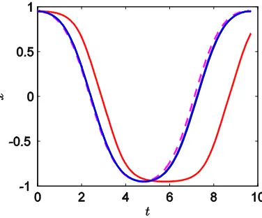
As can be seen, this expression is independent of the coefficient of the linear term α in contrast to (23). The consequence of this is that (25) is less versatile than (19) to accurately approximate the solutions of the Duffing oscillator for all combinations of the coefficients of its terms. In effect, we have noticed that (25) is very poor when

β

=0 as can be observed in Figure 1. Even worse, it becomes completely divergent for some combina-tions of parameters values and oscillation amplitude A. This behavior can be understood by observing that the Fourier series of the residual of (6) with x

( )

τ =Acos

( )

τ and Ω and m given by (14) does not contain the third harmonic. We may conclude that in the HBwL in general, the harmonics to include in the correction to a given stage should be higher than or equal to the least harmonic of the residual terms of that stage. Thus in the re-maining part of this work, we consider only the most versatile expression (19) in our discussion.

To further appreciate the accuracy of the various approximations obtained above, we use the relative error

e a e T T T T T − ∆ ₌ (27)

to compare the approximate period

(

; , ,

)

4

( )

a

K m

T A

w

α β δ = (28)

[image:7.595.219.407.88.244.2]

Figure 1. Comaprison of the approximate solutions to the exact solution for the cubic- quintic Duffing oscillator for

(

α β δ =, ,

) (

1,0, 1−

)

and A=0.95. Solid black line is from exact numerical solution while magenta dashed-line, red solid line and blue solid line correspond respectively to (12), (25) and (19).

(

)

(

)

(

(

)(

)

)

1

2 4 4 2 4 2

0

d

, , 4 6 .

1 3 2 1 6

;

e

y T

y A y A y

A

A

α β δ

δ β δ α

=

− + + + +

∫

(29)

Consider first the case

α β

= =0 and

δ

>0. The exact period can be expressed analytically in terms of the beta function B as

(

)

₂2 1 1 8.413092 ₂

; 0, , 631952725567050114

6 2

, .

0

3

e

T B

A A

A δ δ

δ = _ _=

  (30)

Calculations using the approximate expressions derived above show that the relative errors of the first-order and second-order analytical approximations as compared to the exact solution are respectively less than 0.37% and 0.072%. In comparison it would be necessary to proceed up to the third-order approximation of the standard HBwL to obtain a result just better than our least accurate first-order result; with a relative error of 0.23% [17].

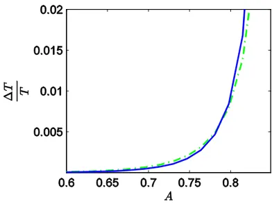
In Figure 2 we compare the relative errors of the single harmonic approximation or cubication, the standard HBwL, and the anharmonic solution when α β δ= = =1. All the three approximations are highly accurate for small values but yet of order O(1) of A. For larger values of the amplitude, the second order approximation of our present approach appears to yield the smallest relative error of 0.072% for the whole range of allowed oscil-lation amplitudes for the parameter values chosen. This last observation concerning large 𝐴𝐴 is the same for all combination of

(

α β,

)

with

δ

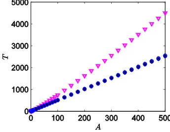
>0.

A further comparison is presented inFigure 3for situations where heteroclinic orbits connecting two distinct equilibrium points exist. Once again we observe that our approach generally provides the best accurate approx-imation. We should point out however that as the oscillation amplitude approaches critically the value for which heteroclinic trajectory is realized, the accuracy of the standard HBwL supersedes our result.

3.2. An Oscillator with Rational Restoring Force

As a second example, we consider a conservative nonlinear oscillatory system in which the restoring force has a rational form. Specifically we choose

( )

2.

1 x f x

x

=

+ (31)

[image:8.595.217.410.85.253.2]

Figure 2. Comparison of the relative errors for the cubic-quintic Duffing oscillator for

(

α β δ =, ,

) (

1,1,1

)

. Green dash-dotted line, magenta dashed-line, and solid blue cor-respond respectively to third order standard HBwL and (12) and (19) of the present work.

Figure 3. Comparison of the relative errors for the cubic-quintic Duffing oscillator for

(

α β δ = −, ,

) (

1, 25 12,1

)

and for amplitude close to the critical value for heteroclinic motion. Green dash-dotted line and solid blue correspond respectively to third order standard HBwL and second order of the present work.

For this form of the restoring force function the expressions of μ and λ in the cubic Duffing equation (17a) approximating (1) with (31) are given by

2 ₂ 4 ₂

1 20 24 1

8 1 ,

1 1

A _A A _A

µ= _ − _+ _ − _

+ +

    (32a)

4 ₂ 6 ₂

8 3 32 1

1 1 .

1 1

A _A A _A

λ= _ − +_ _ − _

+ +

    (32b)

It follows that the expressions of the parameters m and w of the approximate solution of the problem using the method of cubication are

4

2 2 2

2

4 8 3

1 ,

1 1

1 1 .

w

A

A A A

m A

 

= + _ − _

+  + 

= − +

[image:8.595.213.409.318.465.2]

Again these expressions can also be obtained through the lowest order harmonic balance method for (6) with (31). They solve exactly the coefficients of the fundamental and third order harmonics in the residual of this eq-uation when x

( )

τ =Acos

( )

τ . Consequently, the higher order approximation to the solution is taken once again as in (19). It is obvious here that the determination of the Fourier expansion of f x

(

( )

τ

)

is untractable. One can first envisage to expand f x

(

( )

τ

)

in power series of d prior to the computation of the Fourier coefficients. However, upon substituting (19) in (6) with (31), it is simple to reduce it to the same denominator and consider only its numerator. Then by considering the coefficients of cos

( )

τ , cos 3

( )

τ and cos 5

( )

τ we find after some algebraic manipulations that

(

)

4

2 4 ,

3 128 132 19

A d

A A

=

+ + (34a)

(

)

(

)

2 2 2 2

2 3 2 2 2 2

6 32 17 34 8

,

39 45 96 30

d A A d A d

m

A d A d A d A

+ − +

=

− + + − (34b)

and

(

)

(

2 3 2 2 2 2

)

2

4 39 45 96 30

;

w

A d A d A d A

w

A D

− + + −

= (34c)

with

(

) (

)

(

)

2 5 2 4 2 3 2 2 2 2

2511 2157 3804 1509 1188 600 12 6 4 3 .

w

D = A d + A d + − A d + + A d + − A d− − A (34d)

To appreciate the accuracy of the two approximate results in (33) and (34) we have plotted inFigure 4the cor-responding period calculated as 4K m

( )

w and the exact period

( )

(

) (

)

1

2 2 2

0

d 4

ln 1 ln 1

e

y

T A A

A A y

=

+ − +

∫

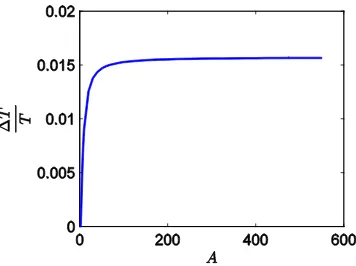
(35)

as a function of A. It appears clearly from this figure that the result obtained from the method of cubication so diverges from the exact result for large oscillation amplitudes that it can simply be considered invalid. However a good match is observed between the result of our proposed approach and the exact result. Figure 5indicates that the maximum relative error on the period is achieved for A→ ∞ and is less than 1.6%.

4. Conclusion and Remarks

[image:9.595.210.382.559.693.2]

In this paper we have investigated the approximation of periodic solutions to autonomous single degree-of- freedom oscillators equations using the Jacobian elliptic function with the objective of improving the method of cubication. To this end we have shown that the properties of these functions can be exploited to put such ODEs

[image:10.595.209.387.86.219.2]

Figure 5.Relative percentage error on the period for the rational restoring force os-cillator.

in a form for which the standard HB and like methods can be applied, while the result is however expressed in terms of Jacobian elliptic functions. Our investigation reveals that in the HBwL the harmonics to include in the correction to a given stage should be higher than or equal to the least harmonic of the residual terms of that stage. With the change of variable sustaining our approach, the analysis can be carried out to higher order, just as in the standard HBwL. For our examples, comparison to the standard harmonic balance indicates that our approach is generally the best, except for periodic orbits too close to a heteroclinic orbit. However, even in this case, the standard HBwL has to be carried to higher order than our approach to gain this advantage. Such a higher order analysis can be quite intricate for non polynomial restoring force. A further interesting property of the solution resulting from our approach is that it also approximates all the harmonics of the exact solution. While the me-thod of rational harmonic balance and the meme-thod of cubication also offer solutions with this property, they do not include a mean to carrying the approximations to higher orders as in the present work. In fact our method encompasses the method of cubication which is equivalent to ist first order application.

References

[1] Wu, B.S. and Li, P.S. (2001) A Method for Obtaining Approximate Analytical Periods for a Class of Nonlinear Oscil-lators. Meccanica, 36, 167-176. http://dx.doi.org/10.1023/A:1013067311749

[2] Wu, B.S. and Lim, C.W. (2004) Large Amplitude Non-Linear Oscillations of a General Conservative System. Interna-tional Journal of Non-Linear Mechanics, 39, 859-870. http://dx.doi.org/10.1016/S0020-7462(03)00071-4

[3] Wu, B.S., Sun, W.P. and Lim, C.W. (2006) An Analytical Technique for a Class of Strongly Non-Linear Oscillators.

International Journal of Non-Linear Mechanics, 41, 766-774. http://dx.doi.org/10.1016/j.ijnonlinmec.2006.01.006

[4] Yamgoué, S.B. and Kofané, T.C. (2008) Linearized Harmonic Balance Based Derivation of the Slow Flow for Some Class of Autonomous Single Degree of Freedom Oscillators. International Journal of Non-Linear Mechanics, 43, 993- 999. http://dx.doi.org/10.1016/j.ijnonlinmec.2008.05.001

[5] Yamgoué, S.B. (2012) On the Harmonic Balance with Linearization for Asymmetric Single Degree of Freedom Non-Linear Oscillators. Nonlinear Dynamics, 69, 1051-1062. http://dx.doi.org/10.1007/s11071-012-0326-1

[6] Nayfeh, A.H. and Mook, D.T. (1979) Nonlinear Oscillations. Wiley, New York

[7] Yuste Bravo, S. (1991) Comments on the Method of Harmonic Balance in Which Jacobian Elliptic Functions Are Used.

Journal of Sound and Vibration, 145, 381-390. http://dx.doi.org/10.1016/0022-460X(91)90109-W

[8] Yuste Bravo, S. (1992) “Cubication” of Non-Linear Oscillators Using the Principle of Harmonic Balance. Internation-al JournInternation-al of Non-Linear Mechanics, 27, 347-356. http://dx.doi.org/10.1016/0020-7462(92)90004-Q

[9] Nayfeh, A.H. (1973) Perturbation Method. Wiley, New York.

[10] Amore, P. and Aranda A. (2003) Presenting a New Method for the Solution of Nonlinear Problems. Physics Letters A, 316, 218-225. http://dx.doi.org/10.1016/j.physleta.2003.08.001

[11] Pelster, A., Kleiner, H. and Schanz, M. (2003) High-Order Calculation for the Frequency of Time-Periodic Solutions.

Physical Review E, 67, Article ID: 016604. http://dx.doi.org/10.1103/PhysRevE.67.016604

[13] Abramowitz, M. and Stegun, I.A. (1972) Handbook of Mathematical Functions. Dover, New York.

[14] Gradshteyn, I.S. and Ryzhik, I.M. (2000) Table of Integrals, Series, and Products. 6th Edition, Academic Press, San Diego.

[15] Mickens, R.E. (2002) Fourier Representations for Periodic Solutions of Odd-Parity Systems. Journal of Sound and Vi-bration, 258, 398-401. http://dx.doi.org/10.1006/jsvi.2002.5200

[16] Beléndez, A., Méndez, D.I., Fernandez, E., Marini, S. and Pascual, I. (2009) An Approximate Solution to the Duff-ing-Harmonic Oscillator by a Cubication Method. Physics Letters A, 373, 2805-2809.

http://dx.doi.org/10.1016/j.physleta.2009.05.074

[17] Lai, S.K., Lim, C.W., Wu, B.S., Wang, C., Zeng, Q.C. and He, X.F. (2009) Newton-Harmonic Balancing Approach for Accurate Solutions to Nonlinear Cubic-Quintic Doffing Oscillators. Applied Mathematical Modelling, 33, 852-866.