Optimizing Hyper Parameters for Improved Diabetes Prediction

(1)

Optimizing Hyper Parameters for Improved Diabetes Prediction

Shaksham Kapoor

1

_{, Krishna Priya S}

2

1

_{Researcher, Imarticus Learning, Pune, Maharashtra, India}

2

_{Assistant Professor, Singhad Institute of Management and Computer Applications, Pune, Maharashtra, India}

---*---Abstract -**

Diabetes also referred to as diabetes mellitus is a long-term condition that causes high blood sugar levels in an individual. The elevated blood sugar levels can damage the body in ways unimaginable, starting from infection risk, skin complications, heart diseases, strokes, kidney damage, nerve damage, blindness etc. Hence, correct diagnosis of diabetes mellitus is an important classification problem, the results of which will have a tremendous impact in the medical field. The purpose of this study is to emphasize the importance of hyper-parameter tuning in improving the accuracy of data mining results. The results obtained were compared with KNN and ANN techniques recently proposed by other researchers and we came to a conclusion that tuning hyper-parameters can increase the accuracy of the model.

Key Words

:

Artificial Neural Network, K-Nearest

Neighbours, Gradient Boosting Trees, Hyper Parameters, Cross-Validation, Stratified Sampling.

1. INTRODUCTION

The word ‘insulin’ is a nightmare for people suffering from diabetes. Diabetes can occur when the pancreas produces very little insulin or no insulin or when the body is not properly responding to insulin. People with diabetes have to maintain their lifestyle and food habits in order to deal with the disease. The most common type of diabetes is: type 1, type 2 and gestational diabetes, less common type of diabetes are monogenic diabetes and cystic fibrosis-related diabetes.

According to International Diabetes Federation, there are 425 million people suffering from diabetes worldwide and 72 million cases exist in India by 2017 which is estimated to rise to 151 million by 2045[1]. Another report from WHO states that India tops the list of the countries with the highest number of diabetes with China, America, and Indonesia follow [2]. Although early detection of diabetes and its treatment is an important step many times the disease is first detected 7 to 10 years after the onset resulting in serious complications such as heart stroke, blindness, kidney failure etc. This is especially the case with type 2 disease which occurs in adults aged over 45 with the highest precent occurring in adults 60 years or older. [3]

Data mining has become a fundamental addition to computing applications in the medical field. Various data mining techniques have helped to understand the medical data clearly, by visualizing or by finding some complex/hidden patterns or diagnosing different features among patients. Many data mining techniques have been

proposed over time by researchers predicting diabetes at an early stage. In our work, we have also proposed an effective data mining technique for early prediction of diabetes. The main focus of our work is to optimize hyper-parameters to improve the accuracy of already proposed models.

2. Literature Survey

[4] Explored the early prediction of diabetes using GMM, SVM, Logistic Regression, ELM and ANN of which ANN showed more accuracy than other techniques. A survey of the various classification techniques is compiled in [5]. The paper also compares the accuracy and SVM showed higher accuracy.

Decision tree induction and SVM are compared to predict diabetes in [6] using WEKA. Paper [7] used five free available data mining and knowledge discovery tools such as WEKA, Rapid miner, Tanagra etc. to compute the accuracy of classification algorithm like Decision tree, Decision Stump, K-Nearest Neighbor and Naïve Bayes algorithm have been compared.

Paper [8] developed a decision tree-based model integrating genetic and clinical features in a gender-specific classification using decision tree, random forest, Naïve Bayes, and support vector machine for the identification of diabetic nephropathy among type 2 diabetic patients.

Paper [9] Naïve Bayes, RBF Network and J48 algorithms are used to for the diagnosis of diabetes using Weka of which Naïve Bayes achieved higher accuracy. A new algorithm which combines KNN with genetic algorithm for effective classification of heart disease is proposed in paper [10]

Paper [11] proposed a weighted fuzzy rule-based clinical decision support system (CDSS) for computer-aided diagnosis of the heart disease. They used a risk prediction method that contains two steps the generation of weighted fuzzy rules and developed a fuzzy rule-based decision support system. The experimentation was carried out on the UCI machine learning repository and the results in risk prediction ensured that the proposed clinical decision support system improved significantly compared with the network-based system in terms of accuracy, sensitivity and specificity.

(2)

accuracy verification.

The paper [13] has investigated 42 demographic and clinical features for 32,555 patients of the FIT Project who were non-diabetic at baseline and took the stress mill test; then they were followed up for five years. They used SMOTE technique which showed significant improvement on the prediction of all classification models prediction performance in line with the gradual increase of the percentages used. They used Random Forest, NB Tree models and to further enhance the prediction accuracy, they used an ensemble method, specifically with the “Vote” technique that combined three decision tree classification methods (Random Forest, NB Tree, and LMT).

A deep learning paradigm based on a solid mathematical theory as well as domain knowledge to predict diabetic glucose is proposed in paper [14]. In this paper, they have demonstrated an example where domain knowledge can be used to build an appropriate compositional structure, leading to a parsimonious deep learning design.

3. Methods

In this paper we have used three different techniques to understand the importance of hyperparameter tuning, they are K-nearest neighbors, Gradient Boosting Classifier and Artificial Neural Networks. Let’s discuss them

KNN: It is a non-parametric, supervised machine learning algorithm which is used for classification problems. Here, non-parametric means that it does not make any assumptions about the underlying data distribution and supervised means, the data is trained with both predictors and response. For a given vector of predictor values, a corresponding response is also present. In simpler cases, the response will either be 0 or 1, leading to a binary classification problem, but KNN can work well with multiple response values as well.

[image:2.595.388.484.140.253.2]

Any set of observation is assigned to a class (0 or 1) most common amongst its K nearest neighbors calculated by a distance function. For continuous numeric data, the distance functions used [15] are shown in Fig -1: -

Fig - 1: Distance metric for Continuous Data

Most commonly used is Euclidean distance, but for categorical data Hamming distance is used [15] as shown in Fig - 2.

Fig - 2: Distance metric for Categorical Data

Having a mixture of categorical and numeric data brings up an issue of standardizing the data between 0 and 1 before the model is trained. Finding optimal value for ‘k’ is not easy, smaller k-values means noise will have a higher influence on your results, while extremely large k-values may lead to under-fitting the data or it may become computationally expensive.

Gradient Boosting Classifier: It is a generalization of the Ada Boost Classifier where the objective was to minimize the loss by using a procedure similar to gradient descent. The following steps are involved: -

Fit an ensemble of models in ∑t p * h(x) a forward stage

manner.

At each stage, add a weak learner compensating the drawbacks of existing weak learners.

These “drawbacks” are identified by gradients, while in Ada Boost they are identified by high-weight data points.

A weak learner has a performance slightly better than average but it can be improved. In gradient boosting classifier, a group of weak learners is ensemble together (compensating each other’s shortcomings) thereby acting as a strong learner. How gradient boosting classifier works for classification problems: -

Step 1. Start with initial models Fa, Fb, Fc, --- Fz, where a,

b, c ---, z represents different classes.

Step 2. Iterate until convergence: -

Calculate negative gradients for class A: -ga(xi) = Ya(xi) – Pa(xi)

Calculate negative gradients for class B: -gb(xi) = Yb(xi) – Pb(xi)

And so, on till,

Calculate negative gradients for class Z: -gz(xi) = Yz(xi) – Pz(xi)

Step 3. Fit regression tree ha to negative gradients:

[image:2.595.75.250.601.744.2]

(3)

-gb (xi)

And so, on till

Fit regression tree hz to negative gradients:

-gz (xi)

Step 4. Fa = Fa + pa * ha

Fb = Fb + pb * hb

And so, on till Fz = Fz + pz * hz

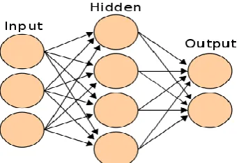
[image:3.595.331.546.122.231.2]

Artificial Neural Networks: Let’s take a look at a simple neural network [16]. shown in Fig – 3

Fig - 3: Simple Neural Network

Suppose we are working on a classification problem which has 2 outputs (0 and 1), we have been given a set of inputs (3 in this case) and a hidden layer with 4 neurons. The most important part here is to determine the weights which will be placed on each link connecting one neuron to another. Here is how ANN does this: -

a. Randomly initialize weights at each link.

b. Using an activation function find the activation value of hidden nodes (input => hidden layer).

c. Using the activation value of hidden nodes, find the activation value of output node using another activation function. (hidden nodes => output).

d. Find the error at the output node using a loss function.

e. Adjust the weights of links between output and hidden layer by calculating the derivatives with respect to weight at each neuron and then updating accordingly.

f. Repeat step (e). for the links between hidden layer and inputs.

g. Repeat steps (a) – (f) till the convergence criteria is met.

The process followed in steps (e) and (f) is also known as “Back Propagation”. There are many different activation functions like tanh, ReLU, sigmoid etc. which are used at both hidden layer and output layer, most commonly used ones are ReLU and sigmoid.

[image:3.595.78.250.248.365.2]

The proposed model in this paper looks similar to this [17], depicted in Fig - 4: -

Fig - 4: Representation of Proposed Neural Network

Cross Validation: A method for evaluating the performance of the model by splitting the dataset into a training set, used for training the model and testing set, used to evaluate the model it.

In k-fold cross-validation, the dataset is randomly divided into k-samples. Of the k-samples, one sample is kept as testing set while the other (k-1) are used as training set. The model is first trained on (k-1) sets and then evaluated on the remaining set, this process is then repeated k times, thereby making every sample a testing sample once. In the end, we have k different evaluation values which can then be averaged to get the final estimate. Title and Author Details

Stratified Sampling: In classification problems, when splitting the dataset into a training set and testing set, there are chances that observations from one class are more than the observation from another class either in training/testing set.

As a result of which, the model will be able to perform well for one set of class predictions and may not work well on another set of class predictions. In order to avoid this, a probability sample is drawn from each group so that the proportion of every output class is similar in both training and testing set.

4. Experiments

4.1 Dataset

For the purpose of this study we have used Pima Indian Diabetes dataset. Given below is the description of the data [18]: -

Pregnancies (preg) Number of times pregnant Numeric Glucose (plas) Plasma glucose concentration a 2

hour in an oral glucose tolerance test

Numeric

Blood Pressure

(press) Diastolic blood pressure (mm/Hg) Numeric Skin Thickness

(4)

Insulin (insulin) 2-hour serum insulin (mu U/ml) Numeric BMI (mass) Body Mass Index (weight in kg /

(height in meter)2) Numeric DPF (pedi) Diabetes Pedigree Function Numeric

Age (age) Age (years) Numeric

Outcome Class variable (0 or 1) Numeric

Total numbers of observations are 768 with 8 numeric columns. Out of 768 observations, 500 tested negative and 268 tested positive.

4.2 Performance Metric

[image:4.595.32.291.80.161.2]

The performance of the model is evaluated by calculating accuracy [19] as given in Fig. 5 which is defined as the sum of correctly classified observations divided by the total number of observations in the test set.

Fig - 5: Evaluation Metric

Where TP, TN, FP, FN are true positive, true negative, false positive and false negative. Every value is determined from the confusion matrix.

4.3 Result and Discussion

[image:4.595.316.552.131.318.2]

The result of our experiments is presented in this section. The experiment has been performed in Python using scikit learn library. Before model building and optimizing the hyper parameters, we did some data visualization to get a sneak peek at the features. From Fig - 6, we can see that some features are right skewed and need pre-processing.

Fig - 6: Histogram depicting right skewness

From Fig - 7, we can see the presence of outliers and they need to treated as well. The last step before model building is standardization of data.

Fig - 7: Boxplots showing outliers

[image:4.595.309.582.420.551.2]

The dataset was then divided into two parts, train set (70% - 536 observations) and test set (30% - 231 observations). The performance of KNN, GBC, and ANN before data pre-processing and after data pre-pre-processing and hyper parameter tuning is described in Table1 and Table 2

Table 1 Performance of algorithms before data pre-processing

[image:4.595.43.280.518.716.2]

(5)

search and Random search. The search was run on a defined range of values for each parameter. The results obtained are cross validated using 3-fold cross validation. For ANN, feature selection was also done using Random forest Classifier, in order to improve the accuracy further.

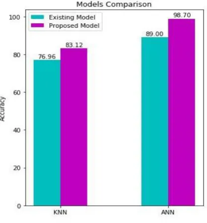
[image:5.595.42.251.284.509.2]

4.4 Comparison with existing models

Fig – 8 shows the comparison of our proposed model with the KNN model proposed by Emrana, Md. Shahid and Md. Rokibul [20]. In the existing model, they have used the value for k (number of nearest neighbors) to be 7. In second case, our ANN model is compared with the ANN model proposed by Komi, Jun Li, Zhai and Zhang [4] in which they have used two hidden layers with 5 neurons in each layer.

Fig - 8: Comparing Models

5. CONCLUSIONS

In this paper, we experimented with optimizing hyper-parameters and tried improving the accuracy of the existing models. The dataset was divided into 70:30 ratio using stratified sampling and the results obtained showed a significant increase in accuracy over existing model [1] where running KNN with 7 neighbors resulted in 76.96 % accuracy on the test set, while the proposed model gave an accuracy of 83.12 % (6.16 % increase). The results obtained with GBC also showed a significant improvement in optimizing hyperparameters. The existing ANN model [2] achieved an accuracy of 89 %, while the optimized model achieved an accuracy of 98.70 % (9.7 % increase).

We came to a conclusion that, optimizing hyper-parameters can have a tremendous effect in improving the accuracy of the model. The optimized model can be used by medical practitioners for detecting diabetes efficiently.

REFERENCES

[1] "Members", Idf.org, 2018. [Online]. Available: https://www.idf.org/our-network/regions-members/south-east-asia/members/94-india.html. [Accessed: 09- May- 2018].

[2] N. Desk, "World Diabetes Day 2017: Number of Diabetics to Double In India by 2023", NDTV.com, 2018. [Online]. Available: https://www.ndtv.com/food/world- diabetes-day-2017-number-of-diabetics-to-double-in-india-by-2023-1775180. [Accessed: 09- May- 2018].

[3] "The Importance of Early Diabetes Detection", ASPE, 2018. [Online]. Available: https://aspe.hhs.gov/report/diabetes-national-plan-action/importance-early-diabetes-detection. [Accessed: 09- May- 2018].

[4] M. Komi, Jun Li, Yongxin Zhai and Xianguo Zhang, "Application of data mining methods in diabetes prediction", 2017 2nd International Conference on Image, Vision and Computing (ICIVC), 2017.

[5] P. Agrawal and A. Dewangan, “A brief survey on the techniques used for the diagnosis of diabetes-mellitus,” Int. Res. J. of Eng. and Tech. IRJET, Vol. 02, pp. 1039-1043, June-2015.

[6] A. Iyer, S. Jeyalatha and R. Sumbaly, “Diagnosis of diabetes using classification mining techniques,” Int. J. of Data M. & Know. Manag.Process, IJDKP, United Arab Emirates, vol. 5, pp. 1-14, January 2015.

[7] A. Naik and L. Samant. “Correlation review of classification algorithm using data mining tool: WEKA, Rapidminer, Tanagra, Orange and Knime,” Int. Con. on Computa. Mod. and Sec., ELSEVIER, Vol. 85, pp. 662-668, 2016.

[8] G.Huang, K.Huang, T.Lee, J. Tzu-Ya and Weng, “An interpretable rulebased diagnostic classification of diabetic nephropathy among type 2 diabetes patients,” Huang et al. BMC Bioinformatics, Vol. 16, pp.55-65, 2015

[9] S. Sa'di, A. Maleki, R. Hashemi, Z. Panbechi and K. Chalabi, "Comparison of Data Mining Algorithms in the Diagnosis of Type Ii Diabetes", International Journal on Computational Science & Applications, vol. 5, no. 5, pp. 1-12, 2015.

[10] M. Jabbar, B. Deekshatulu and P. Chandra, "Classification of Heart Disease Using K- Nearest Neighbor and Genetic Algorithm", Procedia Technology, vol. 10, pp. 85-94, 2013.

(6)

diabetes mellitus — A machine learning approach", 2015 IEEE Recent Advances in Intelligent Computational Systems (RAICS), 2015.

[13]M. Alghamdi, M. Al-Mallah, S. Keteyian, C. Brawner, J. Ehrman and S. Sakr, "Predicting diabetes mellitus using SMOTE and ensemble machine learning approach: The Henry Ford ExercIse Testing (FIT) project", PLOS ONE, vol. 12, no. 7, p. e0179805, 2017.

[14] H. Mhaskar, S. Pereverzyev and M. van der Walt, "A Deep Learning Approach to Diabetic Blood Glucose Prediction", Frontiers in Applied Mathematics and Statistics, vol. 3, 2017.

[15] Saedsayad.com. (2018). KNN Classification. [online]

Available at:

http://saedsayad.com/k_nearest_neighbors.htm [Accessed 9 May 2018].

[16] Simplified!, H., Simplified!, H. and Srivastava, T. (2018). How Does Artificial Neural Network (ANN) Works? Simplified!. [online] Analytics Vidhya. Available at: https://www.analyticsvidhya.com/blog/2014/10/ann-work-simplified/ [Accessed 9 May 2018].

[17] Brilliant.org. (2018). Artificial Neural Network | Brilliant Math & Science Wiki. [online] Available at: https://brilliant.org/wiki/artificial-neural-network/ [Accessed 9 May 2018].

[18] “Pima Indians Diabetes Database | Kaggle", Kaggle.com, 2018. [Online]. Available: https://www.kaggle.com/uciml/pima-indians-diabetes-database. [Accessed: 09- May- 2018

[19] Images.slideplayer.com. (2018). [online] Available at:http://images.slideplayer.com/24/7027794/slides/slide_ 60.jpg [Accessed 9 May 2018].

[20] Hashi, E., Zaman, M. and Hasan, M. (2017). An expert clinical decision support system to predict disease using classification techniques. 2017 International Conference on Electrical, Computer and Communication Engineering (ECCE).