Mining Spatio Temporal Data of Fatal Accident

Mining Spatio-Temporal Data of Fatal Accident

Aina Musdholifah

Department of Computer Science and Electronic, Universitas Gadjah Mada

Yogyakarta, Indonesia

Siti Zaiton Mohd Hadhim

Universiti Teknologi Malaysia Johor, Malaysia

ABSTRACT

Traffic accidents are an important concern of today’s governments and societies, due to the high cost of human and economical resources involved. Data mining has been proven able to significantly help in improving traffic safety. Among several data mining tasks, clustering technique is mostly applied on spatio-temporal data, especially for the traffic data. A number of traffic related works proposed different clustering techniques for mining the spatio-temporal of traffic accident. However, some difficulties appeared when analyzing these datasets, such as the size of data, the lack of statistical evaluation methods, and interpreting the valuable patterns. With regard to solving this problem, this paper proposes a clustering approach for mining spatio-temporal data of fatal accident using local triangular kernel clustering (LTKC) algorithm. LTKC is kernel-density-based clustering algorithm that has the ability to determine the number of clusters automatically. We also propose three visualization techniques for use to interpret and present the optimal clustering result in an easy-understanding form. From the experimental results, LTKC approach was found to be able to discover responsible clusters within fatal accident data, which had proven by silhouette and Dunn index values close to 1. In addition, using visual techniques, we can state that the clustering results were well-separated and compact clusters.

General Terms

Data Mining, Pattern Recognition, Traffic Accident, Clustering Algorithms.

Keywords

Fatal accident; spatio-temporal data; cluster analysis; data mining.

1.

INTRODUCTION

Traffic accidents are an important concern of today’s governments and societies, due to the high cost of human and economical resources involved. Beshah [1] stated that each year, there was more than 1.2 million deaths and 50 injuries in the world. Thus, analyzing accident reports collected from past accidents can be further in reducing accident severity as well as being used as great interest to traffic agencies and the public at large.

Data mining has been proven able to significantly help in improving traffic safety. Among several data mining tasks, clustering technique is mostly applied on spatio-temporal datasets, especially for the traffic dataset [2]. A number of traffic related works proposed different clustering techniques for mining spatio-temporal of traffic accidents, such as [3] who utilized k-means algorithm for doing spatial clustering to find the typical profiles of traffic accidents, [1] who investigated the role of road-related factors in accident severity using predictive models (i.e., decision tree, naive Bayes, and K-nearest neighbors), [4] who analyzed the spatial

and time stamped of Slovenian traffic accidents by applying hierarchical agglomerative clustering for short time series clustering and minimal spanning tree for spatial clustering, and [2] who utilized another traffic dataset, American freeway network and clustered it using DSNN.

However, several difficulties appeared when analyzing these datasets as reported in [3]. One of the difficulties is that these datasets are huge. As a result, they require high time processing cost. In addition, the results of the hierarchical clustering are subjected to the investigator because of the lack of the statistical evaluation methods. Furthermore, most studies focused on predicting or establishing the critical factors influencing injury severity [1], instead of finding the valuable patterns.

Kernel nearest neighbor is one of the density-based clustering techniques [5] that combine k-nearest neighbor density estimation and kernel density estimation to cluster the dataset. It has the capability to determine the number of clusters automatically by defining the clusters as the denser region than others. Local triangular kernel clustering (LTKC) is a clustering algorithm based on kernel nearest neighbor technique. It utilizes triangular kernel function and locally concept, to enhance the performance of another kernel-nearest-neighbor based clustering technique, such as DBSCAN [6], DENCLUE [7] and KFCM [8].

Furthermore, this paper proposes LTKC for mining spatio-temporal data of fatal accident data. The clustering techniques should be in accordance with the characteristics of spatio-temporal data which are complex, high dimension, and large size. Beforehand, a preprocessing stage was performed to analyze the presence of clusters. Next, to analyze the clustering performance, it was necessary to assess the clustering results using various cluster validation techniques. Furthermore, visualization techniques such as Principal Component Analysis (PCA) [9], parallel coordinates plot (PCP) [10], and cartographic map [11] are proposed in this research to interpret and present the optimal clustering result in an easy-understanding form.

The rest of this paper; section 2 provides a detail of LTKC approach including data preprocessing, LTKC algorithm and design of LTKC approach; section 3 describes experiment conducted and results; section 4 gives conclusions and analysis.

2.

LTKC-BASED APPROACH

understanding on the data and may also provide a partial antidote to the dangerous habit of applying clustering techniques in a careless and uncritical way. In this sub section, graphical method designed for an initial exploration of the spatio-temporal data, is described.

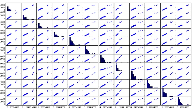
It is often very useful to begin exploration of the spatio-temporal data by examining distributions of each separate variable by way of histograms, boxplots, or non-parametric density estimations, and plots of each pair of variables using a scattergram [12]. Those diagrams may give evidence of patterns or structure in the data, in particular the presence of clusters. Alternatively, they may indicate that the data do not contain distinct groups, thus making the application of clustering less compelling.

A further useful exploration of the data can be obtained from the scattergrams for each variable also [12]. Scattergrams, or commonly called as scatter plot matrix, consists of a number of scatter plots which plot each object of data as point in the plane using the value of two attributes, x and y coordinates [13].

It is helpful to combine the univariate view provided by the Gaussian and bivariate view, provided by scattergrams in the same diagram for initial exploration [12]. It can be used to evaluate the presence of clusters in the dataset. However, this study proposes only a single Gaussian scattergram diagram (SGS diagram) for analyzing the presence of clusters within the spatio-temporal data. SGS diagram combines univariate view presented by the Gaussian density distribution and bivariate view presented by the scattergram.

2.2

Local Triangular Kernel Clustering

Algorithm

This paper proposes clustering algorithm that adopts the clusters in density-based clustering concept. Some reasons of selecting density-based clustering are attributed to its capability to determine the number of clusters automatically by the density of data points in a region cluster [5], to discover clusters with different densities [6] and its relative resistant to noise [13].

The proposed local triangular kernel clustering, LTKC algorithm, assigns objects into clusters using Bayesian decision rule [14]. In the Bayesian decision rule, the class-conditional density that refers to the density of an object is required to be determined. Non-parametric methods of density estimation [15] provide this class-conditional density. However, the proposed LTKC combines k-nearest neighbor (KNN) and kernel density estimation methods.

In this research, the KNN density estimation was extended and combined with kernel function in the kernel density estimation method. Some kernel functions can be used to estimate the density, such as Gaussian and triangular kernel function. However, we used triangular kernel function since it requires less time computation [5]. Hence, the class-conditional density function could be estimated using the combination of KNN density estimation and triangular kernel density estimation. Thus, in the proposed LTKC, the Bayesian decision rule was performed iteratively using this inequality to find the cluster that maximized the density function and assigned the object to the respective cluster. Fig. 1 shows the summary of LTKC algorithm.

2.3

Cluster Visualization

There are many well known visualization techniques in the domain of information visualization. However, in this paper

we propose three visualization techniques to interpret the spatio-temporal clustering result: Scatter-Principal Component Analysis (Scatter-PCA), parallel coordinates plot, and cartographic map. The Principal Component Analysis, PCA originally introduced by [9] and utilized by some researchers such as [16] and [17] as clusters visualization technique, was used in this study to represent the patterns and get an overview of the structure of the whole clusters by visualizing the distribution of data within clusters in 2 dimensional views. Inselberg and Dimsdale [10] introduced parallel coordinates plot, PCP, to analyze the multivariate meanings of each cluster [18]. Besides that, cartographic map [11] is used in this study to analyze the spatial distribution of the spatio-temporal patterns and investigate the location of these patterns.

In this paper, we propose scatter-PCA, that is a combination of PCA and scatter plot. PCA that used SVD matrix decomposition and scatter plot were performed using following steps:

1. Organizing a data set as an m x n matrix, where m is the number of attributes (or measurement) and n is the number of data.

2. Subtracting off the mean for each attribute of object xi. To avoid the data from domination of certain features, use normalization process for PCA approach. This approach started with Z-score data normalization. The objectives of the normalization process were to reduce the square mean error of approximating the input data by data centering and to get unit variance by standardizing the variables (or data scaling). Using Z-score, an attribute value V of an attribute A was normalized to V’ and defined as:

3. Calculating the SVD or the eigenvectors of the covariance to get principal component of the data (PCs).

SVD method of PCA was applied to the normalized dataset to get PC. Applying the PCA to the result of step would provide the the number of PCs obtained as the same with the number of original variables.

4. Eliminating the unnecessary PCs.

To remove the weaker components from this PC set, the variance of PC values and the mean of the variance of PC were calculated. Then, the PCs having variances less than the mean variance was ignoring.

5. Finding the reduced projected data

In the result, the transformation matrix with reduced PCs is formed and this transformation matrix is applied to the normalized data set to produce the new reduced projected dataset.

6. The 2 PCs were plotted using scatter plot

From m-PCs, selects only 2 PCs and plots using scatter plot with different color and symbol for represent different clusters.

polylines, while maintaining the information on each individual dimension and at the same time visualizing the correlations between neighborhood axes.

Scatter-PCA and PCP had been presented in this study for visualizing multidimensional data including spatio-temporal clusters, without considering spatial components. However, in the spatio-temporal clusters obtained by using the proposed algorithm, they contain spatial information that are necessary to be considered for detecting geographic patterns [20]. Mapping is an important method to observe multivariate spatial patterns in the geographic context [21].

This paper presents a method for visualizing the clustering results in cartographic representation [22] of geographic map. Using cartographic map, each data was represented geographically with different colors based on the cluster (produced by TKNN) that contained this item. The resulting cartographic map represented a holistic view of the spatial distribution of discovered multivariate patterns by the proposed algorithm.

We utilized Report Builder 3.0 to create a cartographic map for visualizing the clusters found in fatal accident data. Report Builder 3.0 only required the cluster indices representing the clustering results and geographic map to build a cartographic map. However, we could adjust the distinct colors of region that represent different clusters to get an-easy understanding map.

2.4

Design of LTKC-based Approach

The design of LTKC approach for clustering fatal accident data started with the initial data exploration using SGS diagram analysis to investigate the presence of clusters within the fatal accident data. If the SGS diagram achieved, showed the multimodality of Gaussian distribution that indicated the presence of clusters, then LTKC would be applied to the cluster fatal accident data.

Next, the clustering produced by LTKC was assessed using two index validation measurements, Silhouette [23] and Dunn [24] indices. The optimal clustering, clustering with best Silhouette and Dunn indices, was interpreted using ANOVA analysis to observe the characteristics of each cluster within optimal clustering. These characteristics were then either considered as fatal accident patterns or hidden information.

In addition, to interpret the optimal clustering results visually, scatter-PCA and cartographic map were performed. Fig. 2 shows the design of LTKC-based fatal accident clustering approach. The details of the results and analysis of this experiment will be discussed next section.

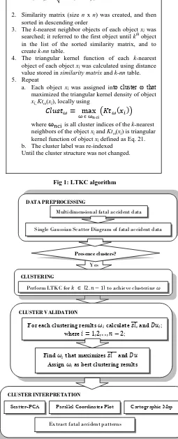
Fig 1: LTKC algorithm

Fig 2: LTKC approach for clustering fatal accident data

DATA PREPROCESSING

Single Gaussian Scatter Diagram of fatal accident data Multidimensional fatal accident data

Yes

Presence clusters?

CLUSTERING

Perform LTKC for to achieve clustering

CLUSTER VALIDATION

For each clustering results calculate _and ; where ;

Find that maximizes and Assign as best clustering results

CLUSTER INTERPRETATION

Scatter-PCA Cartographic Map

Extract fatal accident patterns Parallel Coordinates Plot

1. For each object xi in d-dimension, their Euclidean distance to all objects were calculated,

2. Similarity matrix (size n x n) was created, and then sorted in descending order

3. The k-nearest neighbor objects of each object xi was searched; it referred to the first object until kth object in the list of the sorted similarity matrix, and to create k-nn table.

4. The triangular kernel function of each k-nearest object of each object xi was calculated using distance value stored in similarity matrix and k-nn table. 5. Repeat

a. Each object xiwas assigned into cluster ω that maximized the triangular kernel density of object xi, Ktω(xi), locally using

where is all cluster indices of the k-nearest neighbors of the object xi and Ktω(xi) is triangular kernel function of object xi defined as Eq. 21. b. The cluster label was re-indexed

3.

EXPERIMENTAL RESULTS

3.1

Data Preparation

Traffic accident data used in this study was fatal crash dataset, which was provided by downloaded Fatality Analysis Reporting Systems, FARS [25]. The Fatality Analysis Reporting System, FARS [25] is a national data gathering initiative, sponsored and maintained by the U.S. Department of Transportation National Highway Traffic Safety Administration and is described by [26] and the FARS Coding and Validation Manual [27].

FARS reports records of accidents with fatalities annually, and makes them publicly available under the URL: www-fars.nhtsa.dot.gov. Every accident record is described by groups of attributes referring to various aspects of the accident [28]: accident level, vehicle level, driver level, and person level.

This research used FARS data from 2008 reporting period and is only relevant to the accident level since the objective was to analyze the fatal crashes accident. At the accident level, each record consisted of value of 39 multi-type attributes level [28]. The fatal crash dataset was downloaded from the Fatality Analysis reporting System [25]. The dataset recorded vehicle crashes on public roadway of United States and occurred during January 1994 – December 2008. The fatal crash dataset of each time point was identified within one month, and the data covered 180 time periods from January 1994 to December 2008 and the location of fatal accident identified on 51 states. An event at each time points contained three attributes; fatal accident, vehicle crash, and person. Therefore, the data consisted of 51 spaces, 180 time slots, and 3 non-spatio-temporal attributes.

Since this research only aimed to observe the seasonal effect on fatal crash incidents, only the number of fatal crash incidents values was investigated. As a result, the fatal accident data consisting 51 states and 180 time periods were denoted as rows and columns in the multidimensional

spatio-temporal fatal accident data. Table 1 represents the fatal accident data.

Table 1. The multidimensional fatal accident data

States Number of fatal accidents

Jan-94 Feb-94 … Dec-08

Alabama 78 65 … 72

Alaska 2 6 … 6

. . . … .

. . . … .

. . . … .

Wyoming 9 6 … 13

3.2

Result and Analysis

For prior analysis presence cluster within the fatal accident data, a SGS diagram was created, as shown in Fig.3. Analyzing the sum of number of fatal accidents in each month for all years would be easier if we were to analyze the seasonal effect.

Visually, it is clear that the estimated densities for each pair of two distinct months displayed multimodality, which might be taken as preliminary evidence of the presence of clusters within fatal accident data. All plots indicate very clear clustering in the fatal accident data. Although the presence of clusters within the fatal accident is easy to observed, it is still required to pick out the clusters for extracting pattern within the fatal accident by applying LTKC algorithm.

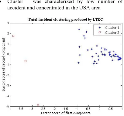
Next, LTKC algorithm was applied to define each cluster that existed within the fatal accident data. From the experimental results, LTKC with k equals to 50 produced the best clustering. The best clustering contained two clusters with average Silhouette index 0.9304 and Dunn index 0.9887. Surprisingly, both validation measurements values were close to 1. It means the best clustering results were very well separated and very compact.

Fig 3: SGS diagaram for fatal accident data

Based on the clustering results obtained by LTKC, there were two clusters of fatal accident data. However, it was necessary

to each clusters using PCP, and location of each clusters spatially using cartographic map. Next, the step was interpreting each cluster obtained as well as extracting the seasonal characteristic and spatial information.

From the experimental results on fatal accident data, LTKC with k equals to 50 had produced the best clustering with two clusters. To observe the distribution of data in each cluster of best clustering, scatter-PCA was performed as shown in Fig. 4. Three of 51 states were clustered in cluster 2 and remaining was clustered in cluster 1.

The map of the spatial fatal accident revealed some striking features. A cartographic map shown in Fig. 5 was created to visualize the location of the fatal accident location of each clusters and furthermore to analyze the neighboring factor. The states within cluster 1 are neighbors to each other and concentrate in the middle of USA area. Meanwhile, cluster 2 contains 3 states, i.e. states California, Florida and Texas. They are located in border of USA.

In some cases, there is no apparent reason why certain states belong to the same cluster. However, some rules were evident. For example, states in Cluster 1 appeared to be in either close to the seaside or in some other way affected by summer migrations (tourism). On the other hand, Cluster 2 had a relatively low traffic activity during the summer months, probably due to a lower effect of tourism on the overall traffic (these clusters mostly included states which are less interesting for tourists, or highly industrial states). In addition, from Fig 5 we can observe that distribution of cluster produced by LTKC was compact. For example, all states in cluster 1 were close and neighbor to each other.

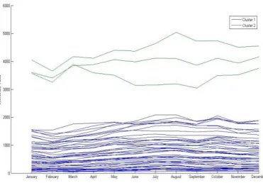
To analyze the seasonal effects that refer to the relationship between attributes, i.e. the month years, PCP was performed, as shown in Fig. 6. From the PCP of fatal accident data, it can be stated that two clusters within the fatal accident data were well separated for all attributes, since there was no overlapping polylines for each attribute of the two clusters.

Next, the patterns or name of the two clusters were defined based on the location of each state within the clusters and the mean of months as shown in Table 2. In this case:

 Cluster 1 was characterized by low number of fatal accident and concentrated in the USA area

 Cluster 2 was characterized by high number of fatal accident and in border of USA. Next, this cluster was considered as a hot spot of fatal accident.

Table 2. The mean and the pattern names of two clusters within fatal accident data

Beat Clusters

Cluster 1 Cluster 2

January 628,75 3743,33

February 576,10 3439,67

March 640,00 3975,67

April 678,17 3868,67

May 751,52 3995,00

June 779,31 3832,00

July 824,23 3974,67

August 835,42 4118,00

September 776,06 3878,67

October 810,08 4119,67

November 745,35 3991,00

December 734,81 4157,33

Patterns Lower number of fatal accident

High number of fatal accidents or hot spot area

Cluster analysis was done for evaluating the presence of clusters in the fatal accident data. To investigate the seasonal effect, a time series of plot of the fatal accident data was also given, as can be seen in Fig.7. It shows that the total number of fatal accidents has not changed much during the period of 15 years. From the data analysis on the fatal accident in USA, the fatal accident was found to decrease during traditional winter (December to February). This was due to the extreme condition, and people were not to go outside. June to August (Summer Season) had high fatal accidents than the winter months, and across the whole year months. A growing number of accidents can be understood as a consequence of more vehicles on the roads, whereas the reasons for less death outcomes might be due to a better traffic infrastructure, safer cars, successful police works, etc.

Fig 4: Structure of clusters on fatal accident data

produced by LTKC Fig 5: A cartographic map of fatal accident clusters in

Fig 6: A PCP of fatal accident attributes Fig 7: A time series plot of fatal accident data

4.

CONCLUSIONS

The LTKC approach for clustering of spatio-temporal data had experimented on the fatal accident data. This approach allows a general framework for clustering in spatio-temporal domain. Our findings show that LTKC algorithm can discover responsible clusters within the fatal accident data, which has been proven by using Silhouette and Dunn index values close to 1. In addition, using visual techniques, we can state that the clustering results were well-separated and compact clusters.

However, the development of computational and visual methods for multivariate spatial analysis has proceeded independently. When development considers both computational and visual methods, the focus will be on sequential application of largely independent methods rather than on developing methods that are integrated from the ground up. In contrast, integrated knowledge discovery environment is needed for further study in extracting hidden patterns within high dimensional spatio-temporal dataset, which is intended to support human interaction for examining the patterns.

5.

ACKNOWLEDGMENTS

This work is supported by a research grant from Universiti Teknologi Malaysia (UTM) VOT number QJ.130000.7128.01H12. The authors gratefully acknowledge many helpful comments by reviewers and members of Soft Computing Research Group (SCRG) UTM Malaysia in improving the publication.

6.

REFERENCES

[1] Beshah, T. and S. Hill. Mining road traffic accident data to improve safety: Role of road-related factors on accident severity in Ethiopia. 2010.

[2] Yin, J., et al. High-dimensional shared nearest neighbor clustering algorithm. 2005. Changsha.

[3] Figuera, C., et al. Multivariate spatial clustering of traffic accidents for local profiling of risk factors. in Intelligent Transportation Systems (ITSC), 2011 14th International IEEE Conference on. 2011.

[4] Lavrac, N., et al., Mining spatio-temporal data of traffic accidents and spatial pattern visualization. Metodoloski zveski, 2008. 5(1): p. 45-63.

[5] Tran, T.N., R. Wehrens, and L.M.C. Buydens, KNN-kernel density-based clustering for high-dimensional multivariate data. Computational Statistics & Data Analysis, 2006. 51: p. 513-525.

[6] Ester, M., et al., A density-based algorithm for discovering clusters in large spatial database with noise,

in 2nd International Conference on Knowledge Discovery and Data Mining. 1996.

[7] Hinneburg, A. and D.A. Keim. An efficient approach to clustering in large multimedia databases with noise. in The fourth international conference on knowledge discovery and data mining (KDD'98). 1998. Menlo Park, CA: AAAI Press.

[8] Zhang, D. and S. Chen. Kernel-based fuzzy and probabilistic c-means clustering. in The International Conference on Artificial Neural Networks. 2003. Istanbul, Turkey.

[9] Hotelling, H., Analysis of a complex of statistical variables into principal components. Journal of Educational Psychology, 1933. 24: p. 417–441.

[10]Inselberg, A. and B. Dimsdale. Parallel coordinates: A tool for visualizing multi-dimensional geometry. in IEEE Visualization. 1990.

[11]Tobler, W., Am Cartogr, 1979. 6: p. 101-106.

[12]Everitt, B.S., Cluster Analysis. 3rd ed. 2000.

[13]Tan, P.N., M. Steinbach, and V. Kumar, Introduction to Data Mining. 2006: Addison Wesley.

[14]Knorr-Held, L. and G. Raber, Bayesian detection of clusters and discontinuities in disease maps. Biometrics, 2000. 56(1): p. 13-21.

[15]Fukunaga, K. and L. Hostetler, The estimation of the gradient of a density function, with applications in pattern recognition. Information Theory, IEEE Transactions on, 1975. 21(1): p. 32-40.

[16]Hoffman, F.M., et al. Multivariate Spatio-Temporal Clustering (MSTC) as a Data Mining Tool for Environmental Applications. in iEMSs 2008:International Congress on Environmental Modeling and Software Integrating Sciences and Information Technology for Environmental Assessment and Decision Making. 2008: International Environmental Modeling and Software Society (iEMSs).

[17]Das, S., M. Lazarewicz, and L.H. Finkel. Principal Component Analysis of Temporal and Spatial Information for Human Gait Recognition. in The 26th Annual International Conference of IEEE EMBS. 2004. San Francisco, CA, USA: IEEE.

[18]Zhou, H., et al., Visual Clustering in Parallel Coordinates. Journal Compilation, 2008. 27(3).

[20]Guo, D., et al., Multivariate Analysis and Geovisualization with an Integrated Geographic Knowledge Discovery Approach. Cartographic and Geographic Information Science, 2005. 32(2): p. 113-132.

[21]Skupin, A., The world of geography: Visualizing a knowledge domain with cartographic means. 2004, PNAS. p. 5274-5278.

[22]Gorricha, J. and V. Lobo, Improvements on the visualization of clusters in geo-referenced data using Self-Organizing Maps. Computers and Geosciences, 2012. 43: p. 177-186.

[23]Rousseeuw, P.J., Silhouettes: A graphical aid to the interpretation and validation of cluster analysis. Journal of Computational and Applied Mathematics, 1987. 20(C): p. 53-65.

[24]Bezdek, J.C. and J.C. Dunn, Optimal Fuzzy Partitions: A Heuristic for Estimating The Parameters in A Mixture of

Normal Distributions. IEEE Transactions on Computers, 1975. C-24(8): p. 835-840.

[25]NCSA, N.C.f.S.a.A. Fatality analysis reporting system (FARS) web-based encyclopedia. 2004 [cited; Available from: http://www-fars.nhtsa.dot.gov/.

[26]TESSMER, J.M., FARS Analytic Reference Guide 1975 to 2002. 2002, National Highway Traffic Safety Administration, Department of Transportation, Washington, D.C.

[27]FARS, Coding and validation manual (2004) 2004, National Center for Statistics and Analysis, National Highway Traffic Safety Administration, Department of Transportation, Washington, D.C.