Inverse Complex Function Dynamics of Ishikawa Iterates
Rajeshri Rana
Asst. Professor
Applied Science and Humanities
Department
G. B. Pant Engg. College,
Pauri Garhwal
Yashwant S. Chauhan
Asst. Professor
Computer Science & Engg.
Department
G. B. Pant Engg. College,
Pauri Garhwal
Ashish Negi
Asst. Professor
Computer Science & Engg.
Department
G. B. Pant Engg. College,
Pauri Garhwal
ABSTRACT
We explore in this paper the dynamics of the inverse complex function using the Ishikawa iterates. The z plane fractal images generated from the generalized
transformation function
z
(
z
n
c
)
1n
2
are analyzed.Keywords
:. Complex dynamics, Relative Superior Mandelbrot Set, Relative Superior Julia set, Ishikawa Iteration..1. INTRODUCTION
Several programs and papers have used escape-time methods to produce images of fractals based on the
complex mapping
z
(
z
n
c
)
1 , where exponent n is a positive integer. The fractals generated from the self-squared function,z
z
2c
wherez
andc
are complex quantities, have been studied extensively in the literature[I3, 4, 5, 6 & 8]. Recently, the generalizedtransformation function
z
z
n
c
for positive integer values ofn
has been considered by K. W. Shirriff [8]. The z plane fractal images for the function1 n
n
z
z
c
for positive and negative, both integer and non-integer values ofn
have been presented by Gujar et al. along with some conjectures about their visual characteristics[4, 5]. In this paper, we considerthe transformation of the function
z
(
z
n
c
)
1, for2
n
, and analyze thez
plane fractal images generated from the iterations of this function using Ishikawa iteration procedure and analyze the drastic changes that occur in the visual characteristics of the images from n = 2, 3, 4,...2. PRELIMINEARIES
The process of generating fractal images from
1
(
n
)
z
z
c
is similar to the one employed for the self-squared function[10]. Briefly, this processconsists of iterating these function upto N times. Starting from a value
z
0 we obtainz z z z
1, 2, 3, 4,...
by applyingthe transformation
z
(
z
n
c
)
1Definition2.1: Ishikawa Iteration [7]: Let X be a subset of real or complex numbers and
f X
:
X
for
x
0X
, we have the sequences{ }
x
n and{ }
y
n in X in the following manner:(
)
(1
)
n n n n n
y
s f x
s x
1
(
) (1
)
n n n n n
x
s f y
s x
where
0
s
n1
,0
s
n1
andn
s
&n
s
are both convergent to non zero number.Definition 2.2: The sequences n
x
and ny
constructed above is called Ishikawa sequences of iterations or Relative Superior sequences of iterates. We denote it byRSO x s s t
(
0,
n,
n, )
.Notice that
RSO x s s t
(
0,
n,
n, )
withs
n=1 is0
(
,
n, )
SO x s t
i.e. Mann’s orbit and if we place1
n n
s
s
thenRSO x s s t
(
0,
n,
n, )
reduces toO x t( , )0 . We remark that Ishikawa orbit0
(
,
n,
n, )
RSO x s s t
withs
n1 / 2
is relative superior orbit.Now we define Mandelbrot sets for function with respect to Ishikawa iterates. We call them as Relative Superior Mandelbrot sets
Definition 2.3: Relative Superior Mandelbrot set RSM for the function of the form
Q z
c( )
z
nc
, where n = 1, 2, 3, 4… is defined as the collection ofc C
for which the orbit of 0 is bounded i.e.{
:
k(0) :
0,1, 2...}
c
RSM
c C Q
k
is bounded.The collection of points that are bounded, i.e. there exists M, such that
|
Q z
n( ) |
M
, for all n, is called as a prisoner set while the collection of points that are in the stable set of infinity is called the escape set. Hence, the boundary of the prisoner set is simultaneously the boundary of escape set and that is Julia set for Q.Definition 2.4: The set of points RSK whose orbits are bounded under relative superior iteration of the function Q (z) is called Relative Superior Julia sets. Relative Superior Julia set of Q is boundary of Julia set RSK.
2.1 Generation Process: The basic principle of generating fractals employs the iterative formula:
1
( )
n n
z
f z
wherez
0 = the initial value of z, andi
z
= the value of the complex quantityz
at the ith iteration. For example, the Mandelbrot’s self-squared function for generating fractals is:f z
( )
z
2c
, wherez
andc
are both complex quantities.We propose the use of the transformation
function
z
(
z
n
c
)
1 for generating fractal images with respect to Ishikawa iterates, wherez
andc
are the complex quantities and n is a real number. Each of these fractal images is constructed as a two-dimensional array of pixels. Each pixel is represented by a pair of( , )
x y
coordinates. The complex quantitiesz
andc
can be represented as:x y
x y
z
z
iz
c
c
ic
where
i
( 1)
andz
x,c
xare the real parts andy
z
&c
yare the imaginary parts ofz
andc
,respectively. The pixel coordinates
( , )
x y
may beassociated with (
c
x,c
y) or (z
x,z
y).Based on this concept, the fractal images can be classified as follows: (a) c-plane fractals, wherein
( , )
x y
is afunction of (
c
x,c
y)(b) z-plane fractals, wherein
( , )
x y
is a functionof (
z
x,z
y). In the literature, the fractals for n = 2 in z plane aretermed as the Mandelbrot set while the fractals for n = 2 in
c
plane are known as Julia sets [10].2.2 Generating the fractals: Fractals have been
generated from
z
z
n
c
using escape-time techniques, for example by Gujar etal.[4, 5] and Glynn [6].We have used in this paper escape time criteria of Relative
Superior Ishikawa iterates for function
z
(
z
n
c
)
1.Escape Criterion for Quadratics: Suppose that
| |
z
max{| |, 2 / , 2 / }
c
s
s
, then|
| (1
) | |
nn
z
z
and|
z
n|
asn
.So,| | | |
z
c
and| | 2 /
z
s
as well as| | 2 /
z
s
shows the escape criteria for quadratics.Escape Criterion for Cubics: Suppose
1/2 1/2
| | max{| |, (| | 2 / ) , (| | 2 / ) }
z
b
a
s
a
s
then
|
z
n|
asn
. This gives an escape criterionfor cubic polynomials
General Escape Criterion: Consider
1/ 1/
| | max{| |, (2 / ) , (2 / ) }
z
c
s
ns
n then|
z
n|
as
n
is the escape criterion. (Escape Criterion derived in [12]).Note that the initial value
z
0 should be infinity, since infinity is the critical point of 1(
n)
z
z
c
. However instead of starting withz
0= infinity, it is simpler to start withz
1 =c
, which yields the same result. (A critical point ofz
F(z) c
is a point whereF
( )
z
0
). The role of critical points is explained in [1].3.
GEOMETRY
OF
RELATIVE
SUPERIOR MANDELBROT SETS AND
RELATIVE SUPERIOR JULIA SETS:
The fractals generated from the equation
z
(
z
nc
)
1possesses rotational as well as reflection symmetry. As conjectured by Gujar and Bhavsar in [4], the fractals generated with the exponent n are (n+1) way rotationally symmetric.
Relative Superior Mandelbrot sets:
Here we notice that the number of wings in the Relative Superior Mandelbrot sets of inverse function is n + 1,
where n is the power of
z
(
z
nc
)
1.As the value of s tend to 1 and s' tends to 1, the Relative Superior Mandelbrot sets of inverse function converts to the general Mandelbrot sets of inverse function, hence we can say that the Relative Superior Mandelbrot sets of inverse function is the general case of the usual Mandelbrot sets of inverse function.
For quadratic function, we have triangular like structures representing symmetry along X axis. For Cubic function, we have symmetry along both X and Y-axis which also represents reflection as well as rotational symmetry. Similarly for the bi quadratic function, we have reflection as well as rotational symmetry.
Relative Superior Julia sets:
Geometrical analysis of the Relative Superior Julia sets of inverse function shows that the boundary of the fixed point region forms a (n + 1) hypocycloid (A hypocycloid is a curve formed by rolling a smaller circle inside a larger circle and tracing a fixed point on the circumference of the smaller circle). The radius of the outer fixed circle for hypocycloid can be computed
as
| |
z
|
z
n|
, where z satisfies thecondition
| |
z
n
1/(n 1), resulting in a radius of/( 1)
(
n
1)
n
n n . The radius of inner moving circle is|
z
n|
yieldingn
n n/( 1).For each value of c, we can iterate the mapping and test if the resulting sequence of z approaches a cycle. Points leading to a cycle can be colored according to the length of the cycle and the points that never enter the cycle but wander chaotically are colored. Figures[All figures of 6.1, 6.2 & 6.3] shows this process. Here white color regions represent stable points while black colored regions represent unstable points.
Relative Superior Julia sets of inverse function for quadratic function shows triangular symmetry. For cubic function Relative Superior Julia sets shows symmetry along X and Y axes both. Moreover this function also describes reflection and rotational symmetry. The biquadratic function shows us the fascinating results. Here we have central planet with satellite like structures
obtained that represents reflection and rotational symmetry.
4. FIXED POINTS
4.1 Fixed points of quadratic polynomial
Table 1: Orbit of F(z) at s=1 and s’=1 for
(z0=-0.06870369332+0.04414015615i)
Number of
iteration i |F(z)|
Number of
iteration i |F(z)|
1 0.081661 11 0.24478
2 0.24251 12 0.24468
3 0.27198 13 0.24464
4 0.24936 14 0.24467
5 0.23735 15 0.24468
6 0.24377 16 0.24467
7 0.24647 17 0.24467
8 0.24491 18 0.24467
9 0.24422 19 0.24467
10 0.24461 20 0.24467
[image:3.612.314.552.70.636.2]Here we observe that the value converges to a fixed point after 16 iterations
Figure 1. Orbit of F(z) at s=1 and s’=1 for
[image:3.612.66.545.151.738.2](z0=-0.06870369332 + 0.04414015615i)
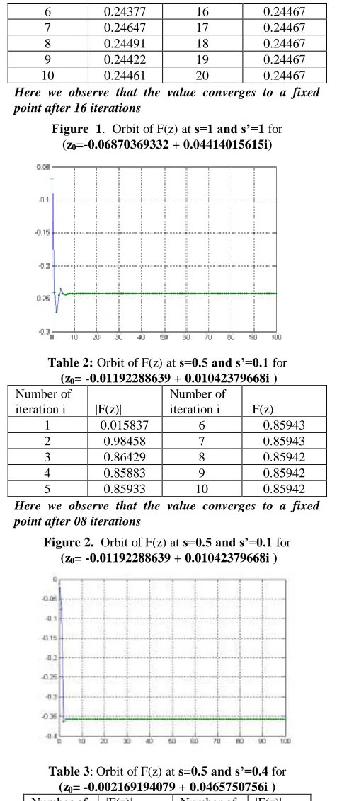
Table 2: Orbit of F(z) at s=0.5 and s’=0.1 for
(z0=-0.01192288639 + 0.01042379668i )
Number of
iteration i |F(z)|
Number of
iteration i |F(z)|
1 0.015837 6 0.85943
2 0.98458 7 0.85943
3 0.86429 8 0.85942
4 0.85883 9 0.85942
5 0.85933 10 0.85942
Here we observe that the value converges to a fixed point after 08 iterations
Figure 2. Orbit of F(z) at s=0.5 and s’=0.1 for
(z0=-0.01192288639 + 0.01042379668i )
Table 3: Orbit of F(z) at s=0.5 and s’=0.4 for
(z0=-0.002169194079 + 0.0465750756i )
Number of iteration i
|F(z)| Number of iteration i
|F(z)|
1 0.046626 11 0.85953
2 0.62449 12 0.85947
3 0.82831 13 0.85944
4 0.85955 14 0.85943
6 0.8626 16 0.85942
7 0.86131 17 0.85942
8 0.86042 18 0.85942
9 0.85991 19 0.85942
10 0.85965 20 0.85942
[image:4.612.74.549.59.750.2]Here the value converges to a fixed point after 16 iterations
Figure 3. Orbit of F(z) at s=0.5 and s’=0.4 for
(z0=-0.002169194079 + 0.0465750756i )
Table 4 Orbit of F(z) at s=0.8 and s’=0.4 for
(z0=-0.01605953579+0.01879439217i )
[image:4.612.78.286.71.128.2] [image:4.612.343.530.445.612.2]Number of iteration i
|F(z)| Number of iteration i
|F(z)|
1 0.024721 7 0.85938
2 1.292 8 0.85943
3 0.76997 9 0.85942
4 0.87184 10 0.85942
5 0.85748 11 0.85942
6 0.85972 12 0.85942
Here the value converges to a fixed point after 09 iterations
Figure 4. Orbit of F(z) at s=0.8 and s’=0.4 for
(z0=-0.01605953579+0.01879439217i )
4.2 Fixed points of Cubic polynomial
Table 1: Orbit of F(z) at s=1 and s’=1 for
(z0=0.01410390589+0.04994371026i)
Number of
iteration i |F(z)|
Number of
iteration i |F(z)|
1 0.051897 5 0.11876
2 0.11758 6 0.11876
3 0.11873 7 0.11876
4 0.11876 8 0.11876
Here we observe that the value converges to a fixed point after 04 iterations
Figure 1. Orbit of F(z) at s=1 and s’=1 for
(z0=0.01410390589+0.04994371026i)
Table 2: Orbit of F(z) at s=0.5 and s’=0.1 for
(z00.00888346751+0.01650347336i)
Number of
iteration i |F(z)|
Number of
iteration i |F(z)|
1 0.018742 6 0.86749
2 0.97928 7 0.86747
3 0.85738 8 0.86747
4 0.86871 9 0.86747
5 0.86732 10 0.86747
Here we observe that the value converges to a fixed point after 07 iterations
Figure 2 Orbit of F(z) at s=0.5 and s’=0.1 for
(z00.00888346751+0.01650347336i)
Table 3: Orbit of F(z) at s=0.5 and s’=0.3 for
(z0-0.02051433067 + 0.012696182776i)
Number of iteration i
|F(z)| Number of iteration i
|F(z)|
1 0.024125 8 0.86716
2 0.7014 9 0.86736
3 0.803 10 0.86743
5 0.85947 12 0.86747
6 0.86474 13 0.86747
7 0.86655 14 0.86747
[image:5.612.68.552.52.743.2]Here the value converges to a fixed point after 12 iterations
Figure 3. Orbit of F(z) at s=0.5 and s’=0.3 for
(z0-0.02051433067 + 0.012696182776i)
Table 4 Orbit of F(z) at s=0.8 and s’=0.3 for
(z0=-0.02051433067+0.01746730516i)
[image:5.612.345.517.151.301.2] [image:5.612.83.272.452.621.2]Number of iteration i
|F(z)| Number of iteration i
|F(z)|
1 0.026943 6 0.86748
2 1.1347 7 0.86747
3 0.81968 8 0.86747
4 0.86911 9 0.86747
5 0.86737 10 0.86747
Here the value converges to a fixed point after 07 iterations
Figure 4. 4 Orbit of F(z) at s=0.8 and s’=0.3 for
(z0=-0.02051433067+0.01746730516i)
4.3 Fixed points of Bi-quadratic polynomial
Table 1: Orbit of F(z) at s=1 and s’=1 for
(z0=-0.6424739888-0.5146558799i)
Number of
iteration i |F(z)|
Number of
iteration i |F(z)|
1 0.82319 5 0.062468
2 0.52011 6 0.062468
3 0.075665 7 0.062468
4 0.062484 8 0.062468
Here we observe that the value converges to a fixed point after 05 iterations
Figure 1 Orbit of F(z) at s=1 and s’=1 for
(z0=-0.6424739888-0.5146558799i)
Table 2: Orbit of F(z) at s=0.5 and s’=0.1 for
(z0=-0.01573769494+ 0.03678871897i )
Number of
iteration i |F(z)|
Number of
iteration i |F(z)|
1 0.040014 8 0.8968
2 0.98215 9 0.89704
3 0.90556 10 0.89699
4 0.88426 11 0.89699
5 0.90308 12 0.89699
6 0.89476 13 0.89699
7 0.8977 14 0.89699
Here we observe that the value converges to a fixed point after 10 iterations
Figure 2. : Orbit of F(z) at s=0.5 and s’=0.1 for
(z0=-0.01573769494+ 0.03678871897i )
Table 3: Orbit of F(z) at s=0.5 and s’=0.3 for
(z0=-0.0227144337+ 0.04376545773i )
Number of iteration i
|F(z)| Number of iteration i
|F(z)|
1 0.049309 11 0.89688
2 0.97756 12 0.89695
3 0.92815 13 0.89698
5 0.89864 15 0.897
6 0.89615 16 0.897
7 0.89585 17 0.89699
8 0.89616 18 0.89699
9 0.89651 19 0.89699
10 0.89675 20 0.89699
[image:6.612.316.541.58.658.2] [image:6.612.74.278.63.475.2]Here the value converges to a fixed point after 17 iterations
Figure 3. Orbit of F(z) at s=0.5 and s’=0.3 for
(z0=-0.0227144337+ 0.04376545773i )
Table 4 Orbit of F(z) at s=0.8 and s’=0.3 for
(z0=-0.008760956177+ 0.05074219649i)
[image:6.612.79.270.482.640.2]Number of iteration i
|F(z)| Number of iteration i
|F(z)|
1 0.051493 9 0.897
2 1.5711 10 0.89704
3 0.68507 11 0.897
4 0.91356 12 0.89699
5 0.93446 13 0.89699
6 0.89932 14 0.89699
7 0.89522 15 0.89699
8 0.8964 16 0.89699
Here the value converges to a fixed point after 21 iterations
Figure 4. Orbit of F(z) at s=0.8 and s’=0.3 for
(z0=-0.008760956177+ 0.05074219649i)
5.
GENERATION
OF
RELATIVE
SUPERIOR MANDELBROT SETS
We present here some Relative Superior Mandelbrot sets for quadratic, cubic and biquadratic function.
5.1 Relative Superior Mandelbrot Sets for Quadratic function:
Figure 1: Relative Superior Mandelbrot Set for s=s'=1
Figure 2: Relative Superior Mandelbrot Set for s=0.8, s'=0.3
Figure 3: Relative Superior Mandelbrot Set for s=0.5,s'=0.1
5.2 Relative Superior Mandelbrot Sets for Cubic function:
Figure 1: Relative Superior Mandelbrot Set for s=s'=1
Figure 3: Relative Superior Mandelbrot Set s=0.5, s'=0.1
[image:7.612.72.541.36.729.2]5.3 Relative Superior Mandelbrot Sets for Bi-quadratic function:
Figure 1: Relative Superior Mandelbrot Set for s=s'=1
[image:7.612.322.542.70.459.2]Figure 2: Relative Superior Mandelbrot Set for s=0.5, s'=0.3
Figure 3: Relative Superior Mandelbrot Set for s=0.5, s'=0.1
6.
GENERATION
OF
RELATIVE
SUPERIOR JULIA SETS:
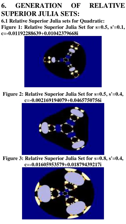
6.1 Relative Superior Julia sets for Quadratic:
Figure 1: Relative Superior Julia Set for s=0.5, s'=0.1, c=-0.01192288639+0.01042379668i
[image:7.612.106.254.70.172.2]Figure 2: Relative Superior Julia Set for s=0.5, s'=0.4, c=-0.002169194079+0.0465750756i
Figure 3: Relative Superior Julia Set for s=0.8, s'=0.4, c=-0.01605953579+0.01879439217i
6.2 Relative Superior Julia sets for Cubic function: Figure 1: Relative Superior Julia Set for s=0.5, s'=0.1,
c=0.00888346751+0.01650347336i
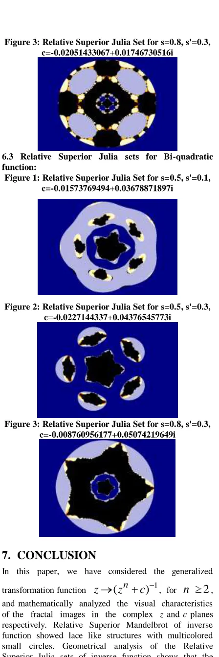
Figure 3: Relative Superior Julia Set for s=0.8, s'=0.3, c=-0.02051433067+0.01746730516i
[image:8.612.90.270.68.190.2]6.3 Relative Superior Julia sets for Bi-quadratic function:
Figure 1: Relative Superior Julia Set for s=0.5, s'=0.1, c=-0.01573769494+0.03678871897i
Figure 2: Relative Superior Julia Set for s=0.5, s'=0.3, c=-0.0227144337+0.04376545773i
Figure 3: Relative Superior Julia Set for s=0.8, s'=0.3, c=-0.008760956177+0.05074219649i
7. CONCLUSION
In this paper, we have considered the generalized
transformation function
z
(
z
n
c
)
1, forn
2
, and mathematically analyzed the visual characteristics of the fractal images in the complex z and c planes respectively. Relative Superior Mandelbrot of inverse function showed lace like structures with multicolored small circles. Geometrical analysis of the Relative Superior Julia sets of inverse function shows that theboundary of the fixed point region forms a (n + 1) hypocycloid. The geometry of Relative Superior Mandelbrot and Relative Superior Julia sets of inverse function showed their rotational as well as reflection symmetry. One of the most fascinating results is the central planet with satellite like structures obtained for biquadratic Relative Superior Julia sets.
8. REFERENCES
[1] B. Branner, The Mandelbrot Set, Proceedings of Symposia in Applied Mathematics39 (1989), 75-105. Published as Chaos and Fractals: The Mathematics Behind the Computer Graphics, ed. R. L. Devaney, L. Keen.
[2] P. Blanchard, Complex Analytic Dynamics on the Riemann Sphere, Bulletin of the American Mathematical Society 11, 1 ( 1984), 85-141. [3] S. Dhurandar, V. C. Bhavsar and U. G. Gujar,
“Analysis of z-plane fractal images from
z
z
c
for α < 0, Computers and Graphics 17, 1 (1993), 89-94.[4] U. G. Gujar and V. C. Bhavsar, Fractals from
z
z
c
in the Complex c-Plane, Computers and Graphics 15, 3 (1991), 441-449. [5] U. G. Gujar, V. C. Bhavsar and N. Vangala,Fractals from
z
z
c
in the Complex z-Plane, Computers and Graphics 16, 1 (1992), 45-49.[6] E. F. Glynn, The Evolution of the Gingerbread Man, Computers and Graphics 15,4 (1991), 579-582.
[7] S. Ishikawa, “Fixed points by a new iteration method”, Proc. Amer. Math. Soc.44 (1974), 147-150.
[8] K. W. Shirriff, “An investigation of fractals
generated by
z
z
nc
”, Computers and Graphics 13, 4 (1993), 603-607.[9] B. B. Mandelbrot, The Fractal Geometry of Nature, W. H. Freeman, New York,1983. [10] H. Peitgen and P. H. Richter, The Beauty of
Fractals, Springer-Verlag, Berlin,1986.
[11] C. Pickover, Computers, Pattern, Chaos, and Beauty, St. Martin’s Press, NewYork, 1990. [12] R. Rana, Y. S. Chauhan and A. Negi, Non
Linear dynamics of Ishikawa Iteration, In Press, Int. Journal of Computer Application (Oct. 2010 Edition).