An efficient algorithm for steepest descent method for unconstrained optimization
14
0
0
Full text
(2) Journal of Science and Technology UTHM. 1.. IntroductIon. Consider the unconstrained optimization problem: min f(x). (1.1). x∈Rn. where f(x) is a continuous differentiable in ℜn. The steepest descent method, which can be traced back to Cauchy (1847) has the following form xk+1 = xk – akgk. (1.2). The search direction gk = g(xk) = ∇f (xk) is chosen as the negative gradient of f at xk and the stepsize ak is given by ak = min f (xk+1). (1.3). a>0. Barzilai and Borwein (1988) proposed stepsize ak that lead to superlinear convergence. Barzilai-Borwein method uses the information in the previous iteration to decide the stepsize in the current iteration. Two stepsizes by Barzilai and Borwein are:. and. sTk yk ak = ––––––– || yk ||22. (1.4). ||sk || 22 ak = ––––––– sTk yk. (1.5). where sk = xk+1 – xk and yk = gk+1 – gk. Barzilai-Borwein method ensures superlinear convergence and performs quite well. Barzilai-Borwein method is not monotone, thus it is not easy to be generalized for general nonlinear functions. A new stepsize enable fast convergence and possesses monotone property is proposed by Yuan (2006). 2 a = ––––––––––––––––––––––––––––––––––––– 2 1 1 4||gk|| 22 1 1 –––– – ––– + –––––––––– + –––– + ––– 2 ak–1 ak ||ak–1 g2k–1||2 ak–1 ak. (1.6). 14. chap 2.indd 14. 15/01/2010 8:58:19 AM.
(3) Journal of Science and Technology UTHM. 2.. A new StepSIze for SteepeSt deScent Method. The new steepest descent method uses the new stepsize after every m exact line search iterations. If m=1, exact line search is use for odd iterations and new stepsize is use for even iterations. Therefore, if m=2, the algorithm has the following form: x2 = x1 – a1 g1 x3 = x2 – a2 g2 x4 = x3 – a3 g3 x5 = x4 – a4 g4 where a1, a2 and a4 are obtained from exact line searches and a3 is obtained from the new stepsize. Algorithm 2.1 : New Steepest Descent Method (m=1) Nonlinear Optimization Step 1 : Given an initial point x1. Compute g1. Set k = 1. Step 2 : Compute the exact line search a2k–1. Set x2k = x2k–1 – a2k–1 g2k–1 Step 3 : If ||g2k|| ≤ TOL, then stop. Step 4 : Compute the exact line searc a2k. Set s2k–1 = x2k – x2k–1 Compute. 2 a2k = ––––––––––––––––––––––––––––––––––––– 2 1 1 4||g2k||22 1 1 –––– – ––– + –––––––– + –––– + ––– a2k–1 a2k ||s2k–1||22 a2k–1 a2k. (1.6). and x2k+1 = x2k – a2k g2k If ||g2k+1||, ≤ TOL then stop. Step 5 : Set k = k + 1 Go to Step 2.. 15. chap 2.indd 15. 15/01/2010 8:58:19 AM.
(4) Journal of Science and Technology UTHM. Algorithm 2.2 : New Steepest Descent Method (m=2) Nonlinear Optimization Step 1 : Given an initial point x1. Compute g1. Set k = 1. Step 2 : Compute the exact line search a3k–2. Set x3k–1 = x3k–2 – a3k–2 g3k–2 If ||g3k–1||, ≤ TOL then stop. Step 3 : Compute the exact line search a3k–1. Set x3k = x3k–1 – a3k–1 g3k–1 If ||g3k||, ≤ TOL then stop. Step 4 : Compute the exact line search a3k. Set s3k–1 = x3k– x3k–1 Compute. 2 a3k = ––––––––––––––––––––––––––––––––––––– 1 1 2 4||g3k|| 22 1 1 –––– – ––– + –––––––– + –––– + ––– 2 a3k–1 a3k ||s3k–1|| 2 a3k–1 a3k. (1.6). and x3k+1 = x3k – a3k g3k If ||g3k+1||, ≤ TOL, then stop. Step 5 : Set k = k + 1 Go to Step 2. According to Algorithm 2.1, exact line search a2k is required for all iterations even though it is only taken in odd iterations. For even iterations, it is used in the calculation of formula (2.1). Stepsize a2k in modified new steepest descent method can be computed without computing the exact line search a2k. Modified new steepest descent method is for convex quadratic functions only is proposed by Yuan (2006). Algorithm 2.3 : Modified New Steepest Descent Method (Quadratic) Step 1 : Given an initial point x1. Compute g1. Set k = 1.. 16. chap 2.indd 16. 15/01/2010 8:58:19 AM.
(5) Journal of Science and Technology UTHM. Step 2 : Compute the exact line search a2k–1. Set x2k = x2k–1 – a2k–1g2k–1 Step 3 : If ||g2k||, ≤ TOL then stop. Step 4 : Set s2k–1 = x2k – x2k–1 s2k = –a2k–1g2k Compute g(x2k + s2k) g(x2k + s2k)T g2k Let β = ––––––––––––– ||g2k||22 Compute. 2 a2k = ––––––––––––––––––––––––––––––––––––– 1 β2 ||g2k||22 –––– (2 – β) + ––––––– + 4–––––– a2k–1 (a2k–1)2 ||s2k–1||22. (2.2). Compute x2k+1 = x2k – a2k g2k If ||g2k+1|| ≤ TOL, then stop. Step 5 : Set k = k + 1 Go to Step 2. Formula (2.2) in modified new steepest descent method and formula (2.1) in new steepest descent method (m=1) is exactly the same if the function is convex quadratic.. 3.. nuMerIcAl reSultS. Numerical performance for steepest descent method (SD), Barzilai-Borwein method (BB) and new steepest descent method (NSD) are compared for nonlinear functions. NSD (m=1) uses exact line search in odd iterations and new stepsize in even two iterations. NSD (m=2) uses the new stepsize after every two exact line search iterations. For quadratic functions, numerical performance for steepest descent method (SD), Barzilai-Borwein method (BB) and modified new steepest descent method (MNSD) are compared. The algorithms are coded in Maple 9. For all problems, the initial point is x1 = (0,0,...,0)T and the stop condition is TOL = 108.. 17. chap 2.indd 17. 15/01/2010 8:58:19 AM.
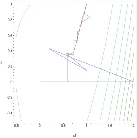
(6) Journal of Science and Technology UTHM. 3.1 1.. Numerical Results for Nonlinear Functions Shalow function f(x1, x2) = (x2 – x12)2 + (1 – x1)2, x(0) = (0, 0)T. Table 3.1 : Numerical Result for Shalow Function x*. Method. Number of Iterations. x1. x2. SD. 153. 0.9999999907. BB. 24. NSD (m=1) NSD (m=2). f(x*). ||g(x*)||. 0.9999999768. 1.08E-16. 9.28E-09. 1.0000000000. 0.9999999998. 1.67E-20. 5.22E-10. 12. 0.9999999986. 0.9999999965. 2.45E-18. 1.30E-09. 10. 1.0000000002. 0.9999999999. 1.88E-19. 2.09E-09. Figure 3.1 : Convergence of iterates for SD method and BB method for Shalow function.. 18. chap 2.indd 18. 15/01/2010 8:58:20 AM.
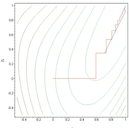
(7) Journal of Science and Technology UTHM. Figure 3.2 : Convergence of iterates for SD method and NSD (m=1) method for Shalow function.. Figure 3.3 : Convergence of iterates for SD method and NSD (m=2) method for Shalow function.. 19. chap 2.indd 19. 15/01/2010 8:58:22 AM.
(8) Journal of Science and Technology UTHM. 2.. Cube function f (x1, x2) = 100(x2 – x13)2 + (1 – x1)2, x(0) = (0, 0)T. Table 3.2 : Numerical Result for Cube Function x*. Method. Number of Iterations. x1. x2. SD. **. 0.5217012703. BB. 1448. NSD (m=1) NSD (m=2). f(x*). ||g(x*)||. 0.1419925334. 2.29E-01. 9.56E-01. 0.9999999849. 0.9999999546. 2.29E-16. 9.62E-09. 220. 1.0000000000. 0.9999999999. 2.08E-21. 8.88E-11. 188. 0.9999999972. 0.9999999915. 8.06E-18. 1.80E-09. Note : **more than 2500 iterations. 1.2 1. f(x). 0.8 0.6 0.4 0.2 0 0. 20. 40. 60. 80. 100. 120. 140. 160. 180. Iterations SD. BB. NSD (m=1). NSD (m=2). Figure 3.4 : Convergence of iterates for SD method, BB method, NSD (m=1) method and NSD (m=2) method for Cube function.. 20. chap 2.indd 20. 15/01/2010 8:58:22 AM.
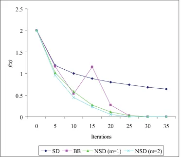
(9) Journal of Science and Technology UTHM. 3.. Rosenbrock Function f (x1, x2) = 100(x2 – x13)2 + (x1 – 1)2 + 100(x4 – x23)2 + (x3 – 1)2 , x(0) = (0,0,0,0)T Table 3.3 : Numerical Result for Rosenbrock Function x*. Method. Number of Iterations. x1. x2. x3. x4. SD. **. 0.990. 0.980. 0.990. BB. 40. 1.000. 1.000. 1.000. NSD (m=1). 40. 1.000. 1.000. NSD (m=2). 35. 1.000. 1.000. 1.000 1.000. f(x*). ||g(x*)||. 0.980. 1.01E-04. 2.01E-02. 1.000. 4.68E-18. 3.66E-09. 1.000. 1.36E-21. 3.34E-11. 2.25E-25. 3.82E-13. 1.000. Note : **more than 2500 iterations. 2.5 2. f(x). 1.5 1 0.5 0 0. 5. 10. 15. 20. 25. 30. 35. Iterations SD. BB. NSD (m=1). NSD (m=2). Figure 3.5 : Convergence of iterates for SD method, BB method, NSD (m=1) method and NSD (m=2) method for Rosenbrock function.. 21. chap 2.indd 21. 15/01/2010 8:58:22 AM.
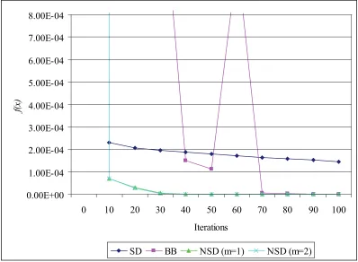
(10) Journal of Science and Technology UTHM. 4.. Powell function f (x1, x2, x3, x4) – (x1 + 10x2)2 + 5(x3 – x4)2 + (x2 – 2x3)4 + 10(x1 – x4)4, x(0) = (0.1, 0..1, 0.1, 0.01)T. Table 3.4 : Numerical Result for Powell Function x*. Method. Number of Iterations. x1. x2. x3. x4. SD. **. 0.03907. -0.00390. 0.01945. 0.01949. f(x*). ||g(x*)||. 4.837E-06. 1.073E-03. BB. 198. 0.00103. -0.00010. 0.00048. 0.00048. 2.158E-12. 7.279E-09. NSD (m=1). 109. 0.00036. -0.00004. 0.00026. 0.00026. 9.243E-14. 9.206E-10. NSD (m=2). 119. 0.00111. -0.00011. 0.00055. 0.00055. 3.076E-12. 9.665E-09. Note : **more than 2500 iterations. 8.00E-04 7.00E-04 6.00E-04. f(x). 5.00E-04 4.00E-04 3.00E-04 2.00E-04 1.00E-04 0.00E+00 0. 10. 20. 30. 40. 50. 60. 70. 80. 90. 100. Iterations SD. BB. NSD (m=1). NSD (m=2). Figure 3.6 : Convergence of iterates for SD method, BB method, NSD (m=1) method and NSD (m=2) method for Powell function.. 22. chap 2.indd 22. 15/01/2010 8:58:22 AM.
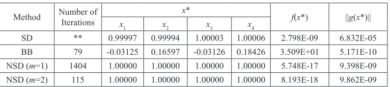
(11) Journal of Science and Technology UTHM. 5.. Wood Function f (x1, x2, x3, x4) = 100(x2 – x12)2 + (1 – x1)2 + 90(x3 – x23)2 + (1 – x3)2 + 10.1[(x2 – 1)2 + (x3 – 1)2] + 19.8(x2 – 1)(x4 – 1) x(0) = (0, 0, 0, 0)T Table 3.4 : Numerical Result for Wood Function x*. Method. Number of Iterations. x1. x2. x3. x4. SD. **. 0.99997. 0.99994. 1.00003. BB. 79. -0.03125. 0.16597. -0.03126. NSD (m=1). 1404. 1.00000. 1.00000. 1.00000. 1.00000. 5.748E-17. 9.398E-09. NSD (m=2). 115. 1.00000. 1.00000. 1.00000. 1.00000. 8.193E-18. 9.862E-09. f(x*). ||g(x*)||. 1.00006. 2.798E-09. 6.832E-05. 0.18426. 3.509E+01. 5.171E-10. Note : **more than 2500 iterations Barzilai-Borwein method could not solve Wood function. 6.. Beale Function f (x1, x2, x3, x4) = 100(x2 – x21)2 + (1 – x1)2 + 90(x4 – x23)2 + (1 – x3)2 + 10.1[(x2 – 1)2 + (x4 – 1)2] + 19.8(x2 – 1)(x4 – 1) x(0) = (0, 0, 0, 0)T x*. Method. Number of Iterations. x1. x2. x3. x4. x5. x6. SD. 302. 3.00. 0.50. 3.00. 0.50. 3.00. f(x*). ||g(x*)||. 0.50. 1.25E-16. 8.85E-09. BB. **. 100.18. 0.99. 100.18. 0.99. 100.18. 0.99. 1.31E+00. 2.65E-04. NSD (m=1). 16. 3.00. 0.50. 3.00. 0.50. 3.00. 0.50. 1.75E-20. 1.04E-10. NSD (m=2). 16. 3.00. 0.50. 3.00. 0.50. 3.00. 0.50. 5.73E-23. 7.49E-11. Note : **more than 2500 iterations Barzilai-Borwein method could not solve Beale function.. 23. chap 2.indd 23. 15/01/2010 8:58:23 AM.
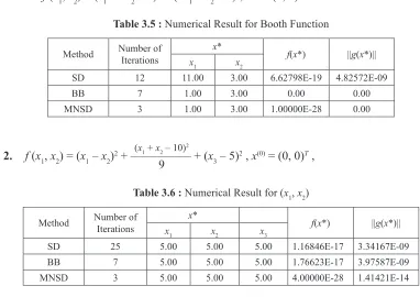
(12) Journal of Science and Technology UTHM. 3.2 1.. Numerical Results for Quadratic Functions Booth function f (x1, x2) = (x1 + 2x2 – 7)2 + (2x1 + x2 – 5)2, x(0) = (0, 0)T Table 3.5 : Numerical Result for Booth Function. 2.. x*. Method. Number of Iterations. x1. x2. SD. 12. 11.00. BB. 7. MNSD. 3. f(x*). ||g(x*)||. 3.00. 6.62798E-19. 4.82572E-09. 1.00. 3.00. 0.00. 0.00. 1.00. 3.00. 1.00000E-28. 0.00. (x + x – 10)2. 1 2 f (x1, x2) = (x1 – x2)2 + –––––––––– + (x3 – 5)2 , x(0) = (0, 0)T , 9. Table 3.6 : Numerical Result for (x1, x2) x*. Method. Number of Iterations. x1. x2. x3. f(x*). ||g(x*)||. SD. 25. 5.00. 5.00. 5.00. 1.16846E-17. 3.34167E-09. BB. 7. 5.00. 5.00. 5.00. 1.76623E-17. 3.97587E-09. MNSD. 3. 5.00. 5.00. 5.00. 4.00000E-28. 1.41421E-14. Barzilai-Borwein method could not solve some nonlinear functions like Wood function and Beale function. The numerical results show that new steepest descent method is better than steepest descent method and Barzilai-Borwein method for many nonlinear functions. Besides that, new steepest descent method (m=2) is better than new steepest descent method (m=1) for many nonlinear problems. The results also show that modified new steepest descent method ensures the solution within 3 iterations.. 4.. dIScuSSIon. Barzilai-Borwein method performs quite well if compared to steepest descent method. However, Barzilai-Borwein method sometimes presents problems because all algorithms of this method have to start at origin. Unlike Barzilai-Borwein method, new steepest descent method and modified new steepest descent method can start at any initial point. The new steepest descent method uses the new stepsize after every m exact line search iterations. In short, new steepest descent method and modified new steepest descent method perform well for many problems. 24. chap 2.indd 24. 15/01/2010 8:58:23 AM.
(13) Journal of Science and Technology UTHM. 5.. referenceS. Barzilai, J. and Borwein, J.M. (1988). Two Point Step Size Gradient Methods. IMA Journal of Numerical Analysis, 8:141-148. Cauchy, A. (1847). Methode generale pour la resolution des systems dequations simultanees. Comp. Rend. Sci. Paris, 25:46-89. Raydan, M. (1993). On the Barzilai and Borwein Choice of Steplength for the Gradient Method. IMA Journal of Numerical Analysis, 13:321-326. Yuan, Y. (2006). A new stepsize for the steepest descent method. Journal of Computational Mathematics, 24: 149-156.. 25. chap 2.indd 25. 15/01/2010 8:58:23 AM.
(14) Journal of Science and Technology UTHM. 26. chap 2.indd 26. 15/01/2010 8:58:23 AM.
(15)
Figure

+4
Related documents
The property of TRSs that guarantees the desired completeness (for ground µ -weakly normalizing and ground confluent TRSs, see [3, Theorem 1]) is called µ - canonical completeness
Management control systems include two variables namely interactive approach (with twelve items) and diagnostic approach (with eight items) as well as contemporary
János Kornai’s Anti-Equilibrium was ahead of its time when it was written, and even today, when system dynamics software is extensively used in engineering and other disciplines,
It should be noted that: (I) An acceptance of the seller’s price and/or exchange rate will not be withdrawn provided the goods presented to SGS inspection conform with the
The transient absorption at 300 nm and ground state bleaching at 360 nm observed at the Al 3+ concentration employed are similar to those observed following irradiation of
Johnson, A., 2006, FDI Inflows to the Transition Economies in Eastern Europe: Magnitude and Determinants, The Royal Institute of Technology, CESIS (Centre for Excellence for Studies
The Readiness for Interprofessional Learning Scale (RIPLS) was adminis- tered to all 2nd-, 3rd-, and 4th-year undergraduate students of the respiratory care, physical therapy,
Previously referred to as a Material Safety Data Sheet (MSDS) an SDS is a docu- ment containing information and instructions on hazardous materials present in the workplace;
