Nontraditional Monetary Policy in a Model of Default Risks and Collateral in the Absence of Commitment

Nontraditional Monetary Policy in a Model of Default

Risks and Collateral in the Absence of Commitment

Hiroshi Fujiki

Faculty of Commerce, Chuo University, Japan

Copyright©2017 by authors, all rights reserved. Authors agree that this article remains permanently open access under the terms of the Creative Commons Attribution License 4.0 International License

Abstract

We show that a central bank could improve the allocation of resources by delivering the defaulting party’s collateral goods to those who consume the most quickly. We base our discussion on Mills and Reed [1]’s repo contract model, which shows that the consumption of the lender will be the same whether the borrower is a productive agent or an unproductive agent. We extend their model by considering shocks to the second period of lenders’ lives, which force them to consume within an early stage of the second period of their lives. The shock could make the consumption of lenders vary depending on the timing of transactions in the goods market. We show that a central bank could make the consumption of lenders constant regardless of the timing of transactions in the goods market, and could achieve better resource allocation by using various nontraditional monetary policy tools.

Keywords

Collateral, Contract, Repurchase Agreement, Nontraditional Monetary Policy

1. Introduction

After the Global Financial Crisis (GFC), financial regulators have been introducing many new measures to achieve financial stability. Those measures, summarized in the Financial Stability Oversight Council Annual Report or Financial Stability Board (FSB) “Strengthening Oversight and Regulation of Shadow Banking: Policy Framework for Addressing Shadow Banking Risks in Securities Lending and Repos,” August 29, 2013, include building high-quality capital, central clearing of over-the-counter (OTC) credit derivatives, and the introduction of a dynamic fails charge in the US repo market. Such measures would certainly make many financial contracts safer compared with those available before the GFC. However, people could face other risks that financial regulators have not dealt with. For example, a middle-aged man could save money by making an investment in a repo contract to prepare for his retirement.

The repo contract would be safer than that available before the GFC, thanks to the efforts of financial regulators. However, when the man becomes old, he may realize that he is going to die soon and has too little time to spend his money, because producers could supply the consumption goods only after his death. Are there any policy measures that can help this unlucky man? If any measures were available, who could have helped this unlucky man? Note that many central banks assumed responsibility for creating financial stability after the GFC. Are there any policy tools, including monetary policy tools, which are useful for addressing those risks?

In this paper, we consider a bilateral repo contract as one of the financial contracts that has become safer thanks to the efforts of financial regulators after the GFC. However, the financial regulators and central bankers have not dealt with the risk that the lender of that repo contract could die soon.

Suppose that one agent, called a central bank, can commit to a socially beneficial policy. We show that a central bank could improve the allocation of resources under such risk by delivering the defaulting party’s collateral goods to those who consume the most quickly, in other words, by encouraging quicker rehypothecation. The welfare gains from this policy arise from the collection and use of public information regarding the outcome of all investment projects based on bilateral repo contracts.

Regarding the lack of commitment, Mills and Reed [1] assume that there is no public record keeping of agent histories and no repeated relationships between a borrower and a lender (and thus no use of punishment mechanisms to encourage a borrower to repay). They also assume that there is no enforcement technology by which collateral can be seized (and thus the collateralized lending should be viewed as a repo contract, because the borrower will need to buy back the collateral by paying money to the lender).

Regarding the role of exogenous idiosyncratic risks, their model assumes that the lender does not have any particular use for collateral value per se. The lender needs fiat money that would allow him to purchase his desired consumption goods at a future date. Thus, the non-defaulted borrower must repay his borrowings to the lender via fiat money, and in the event of the borrower’s default, the lender will sell collateral to obtain fiat money in the secondary market.

The novelty of their model lies in the result that the lack of commitment by both lenders and borrowers generates an additional incentive constraint and that the value of collateral to the lender should not exceed the value of returning the collateral to the borrower. The constraint for the lender may sound unfamiliar; however, it corresponds to so-called “settlement fails” in repo contracts, where the lender intentionally chooses not to return the collateral asset and gives up the principal and interest rate payments from the borrower.

Mills and Reed [1] show that these incentive constraints give rise to the result that the amount of goods obtained by the lender will be the same whether the borrower is a productive agent (not subject to an idiosyncratic default shock) or an unproductive agent (subject to an idiosyncratic default shock). When the borrower is a productive agent, he repays his borrowings by means of fiat money. When the borrower is an unproductive agent and fails to repay his borrowings, the lender will sell the collateral in the secondary market to obtain fiat money. Namely, the collateral serves as insurance against the borrower’s default. Moreover, these incentive constraints lead to a situation where the borrower is not insured against the idiosyncratic default shock to him.

This paper extends Mills and Reed [1] by adding a shock to the lenders’ consumption in the second period of their lives. Thanks to the collateral’s role as insurance against the borrower’s default, the lenders have the same money balances irrespective of the borrower’s default, and thus they consume the same amount of goods in the second period of their lives. However, the lenders, who enter the second period of their lives with the same amount of money, may not enjoy the same level of consumption in the second period of their lives if they are hit by a shock to their consumption, and thus their expected utilities will decrease as the following example.

Suppose that some lenders are hit by a taste shock at the beginning of the second period of their lives, which forces them to consume within an early stage (say, in the morning)

of the second period of their lives. Suppose further that the amount of goods available within an early stage of the second period of their lives is not enough to meet the demand for goods from the lenders hit by a taste shock, while more goods are available on the resale market for collateral goods in the later stages (say, in the afternoon) of the second period of their lives. In that case, the level of consumption in the second period of their lives could vary depending on the timing of their consumption, and their expected utilities will decrease even though they enter the second period of their lives with the same amount of money as the other lenders who are not hit by a taste shock.

Can a central bank improve the allocation of resources in such a situation? This paper argues that if a central bank commits to delivering the defaulting party’s collateral goods to those who consume the most quickly, it can improve the allocation of resources as described below. Note that because we assume limited commitment of private agents, it is reasonable that we assume that only one agent can commit such an action. We call this agent a central bank.

Let us suppose that a central bank can commit the following policy action. Suppose further that within an early stage of the second period of the lives of the old lenders hit by a taste shock, the central bank identifies the young lenders whose borrowers are unproductive agents and thus prepare to sell the collateral goods in the resale market in the later stages of that period. Then, the central bank proposes that those young lenders trade their collateral goods for fiat money held by the lenders who are hit by a taste shock within an early stage of that period.

The welfare gains achieved by the policy action above arise from the collection and use of public information regarding the outcome of all investment projects based on bilateral repo contracts at the beginning of the second stage by a central bank. The central bank knows the return on the risky investment for each bilateral contract and the average default rate, and uses that information to arrange socially beneficial trade between young lenders and old lenders with a taste shock.

The rest of the paper is organized as follows. Section 2 reviews related literature. Section 3 explains the environment and the sequence of events within a period, and Section 4 analyzes the optimal allocations in the absence of commitment. Section 5 discusses possible policy options to improve the allocation of resources, and Section 6 draws conclusions.

2. Related Literature

role of collateral, which Mills and Reed [1] puts emphasis on.

Second, regarding the role of exogenous idiosyncratic risks and the use of collateral, Shi [5] and Mills [6,7] model collateral as repurchase agreements in the absence of commitment. Ferraris and Watanabe [8] allow the possible resale of collateral in the event of default. However, these models do not consider the idiosyncratic risk that leads to default and thus do not study the insurance role of collateral. Third, regarding the additional incentive constraint that the value of collateral to the lender should not exceed the value of returning the collateral to the borrower, Mills and Reed [1] points out that the constraint corresponds to so-called “settlement fails” in repo contracts. We explain “settlement fails” below. As explained in Garbade et al. [9], prior to May 2009, US market convention enabled a seller of US Treasury securities to postpone their obligation to deliver the securities without an explicit penalty. As long as short-term interest rates were above 3% or so, the time value of money usually sufficed to encourage timely settlement. However, the Lehman failure in 2008 caused “flight to quality,” which led to short-term interest rates from 1.5% to zero; this resulted in chronic settlement fails. Under near zero short-term rates, the time value of money no longer provided adequate incentive to settle on time, and an extraordinary volume of fails threatened to erode the perception of the market as free of credit risk. In response, the Treasury Market Practices Group introduced a “dynamic fails charge” in May 2009 to incentivize timely settlement of Treasury securities and reduce fails. Readers can see Copeland and Selig [10] about the development of a fail charge in the US repo market. After the introduction of a dynamic fails charge, the number of settlement fails fell substantially; however, they did not fall to zero. Readers can see data on settlement fails in the US market and possible explanations for the high level of fails in June 2014 in Fleming et al. [11, 12]. This episode shows why we should take the additional incentive constraint for the lender seriously, since it prevents strategic settlement fails by the lender, as proposed by Mills and Reed [1].

Fourth, regarding the welfare gains achieved by the policy action, our model is similar to that of Freeman [13], in which some of the lenders, who are hit by a taste shock, and must depart from the lending market quickly and are forced to sell their loans below par value for fiat money because the available amount of fiat money in the lending market is insufficient. However, the policy implication in our model is quite different from that of Freeman. In the case of Freeman [13], a central bank’s issue of additional fiat money in the resale market of IOUs resolves the lack of liquidity in that market and helps to achieve a better resource allocation. In our model, this traditional policy à la Freeman [13] cannot improve the resource allocation because additional fiat money would not increase the production of good in time for the consumption by the lenders who are hit by a taste shock. The welfare gains

achieved by the policy action in our model arise from the collection and use of public information regarding the outcome of all investment projects based on bilateral repo contracts at the beginning of the second stage by a central bank. The central bank knows the return on the risky investment for each bilateral contract and the average default rate, and uses that information to arrange socially beneficial trade between young lenders and old lenders with a taste shock.

Fifth, the benefit achieved by the intervention by the central bank in our model is related to the information advantage of using a central counter party (CCP) to clear the OTC financial contracts. A CCP has access to the specifics of all contracts, and can gather information and release useful aggregate statistics on the prices and quantity of the contracts, as Monnet [14] suggested. It is true that a coalition of lenders, such as a private CCP, could also improve the allocation of resources as Green [15] points out in the context of the policies suggested by Freeman [13] in practice. However, since we assume limited commitment of private agents, it is reasonable that we assume that only one agent can commit such an action, hence we do not call that agent as CCP. One may also argue that a blockchain, say public ledger of all transactions of collateral goods, would allow the collection and use of public information regarding the outcome of all investment projects based on bilateral repo contracts. However, in this paper we assume there is no public record of agent’s trading histories. In general, the division of labor between private institutions and public institutions is one of the issues beyond the scope of this paper because the model in this paper assumes that there is no public record keeping of agent histories and no repeated relationships between a borrower and a lender. These assumption prevent us from making a particular policy recommendation for some economic institutions.

Their second arrangement relaxes the incentive constraints, which prevents defaulting agents from taking the collateral pledged by their counterparty and walking away from the contract, and thus improves welfare. In our model, the central bank operates as a type of rental warehouse to store the collateral, and does not have the enforcement power to prevent the strategic default of a lender, and thus does not relax the incentive constraints for strategic default by the lender. Moreover, only the borrowers submit collateral in our model, while both parties in the bilateral contract submit collateral as in Monnet and Nellen [16].

3. Environment and Trading Patterns

3.1. The Environment

This section explains our model, which extends that of Mills and Reed [1] by adding a friction where some lenders are hit by a taste shock at the beginning of the second period of their lives that forces them to consume within an early stage of the second period of their lives.

The economies start at period 1, and agents live for two periods. We call the agents “young agents” in the first period of their lives, and “old agents” in the second period of their lives. There are two types of agents who have different endowments when they are born. Each type-A agent is endowed with x units of good α when young and nothing when old, and each type-B agent is endowed with y units of good β when young and nothing when old.

Let aZtt′ denote consumption of good z at date t′ of a type-A agent of generation t. The utility functions of a type-A agent are ( , t )

t t

t

A _{a a}

u α β . The functions uA are strictly increasing and concave in each argument; this satisfies the Inada conditions. Note that type-A agents consume their own endowment good and type B’s endowment good when young, and type-A agents consume nothing when old.

Let t t Z

b ′ denote consumption of good z at date t′ of a type-B agent of generation t. The utility of a type-B agent depends on his consumption of his endowment when young and his consumption of the good endowed to a type-A agent when old. We depart from Mills and Reed [1] in one respect: we assume that a type-B agent’s timing of consumption of the good endowed to a type-A agent when old is determined randomly by a taste shock when he becomes old. In particular, a type-B agent consumes the good endowed to a type-A agent in an early stage of his old age with probability D, and in any stage of his old age with probability (1–D). A type-B agent’s expected utility function at date t is uB(bβtt,bαt,t+1).

In addition to the endowments of two types of goods, there are two agent-specific storage technologies involving goodsα . Type-B agents have access to perfect storage technology within a period. Type-A agents have productive yet risky technology. With probability η, their investments

generate nothing. With probability 1–η, their investments generate R units of goodsα. On average, the investment technology generates higher returns than the storage technology, and thus R (1–η) > 1.

In period t = 1 there is a [0, 1] continuum of initial old type-B agents. They are endowed with M divisible units of national fiat money.

3.2. Sequence of Events within a Period

We explain the sequence of events within a period. Each period t is divided into four stages, which are explained below. The sequence of events within the second stage differs from that of Mills and Reed [1].

3.2.1. The First Stage

In the first stage, each generation-t type-A agent is matched with a generation-t type-B agent. Two activities can take place at these meetings. The first is a potential transfer of some of the good β from the type-B agent to the type-A agent. The second is an allocation of good αinto the two agent-specific technologies. An amount σ ≤x can be transferred from the type-A agent to the type-B agent to be allocated to safe storage technology. The remaining amount

σ

−

x is then invested in the type-A agent’s risky technology. We assume that good β perishes at the end of this stage, so this is the only opportunity for a type-A agent to acquire and consume some of good β. Both agents consume their allocation of good β before the end of the first stage.

3.2.2. The Second Stage

At the beginning of the second stage, the return on the risky investment is realized. Unlike Mills and Reed [1], after the realization of risky investment, some generation-(t–1) type-B agents are hit by a taste shock that forces them to consume good α within an early stage (say, in the morning) of the second period of their lives. Specifically, the fraction D of generation-(t–1) type-B agents trade in the second stage and consume quickly, as supposed by Freeman [13]. Hereafter, we call them “early-departing type-B agents”. Suppose further that the fraction (1–D) of generation-(t–1) type-B agents trade in both the second stage and in the fourth stage. Hereafter, we call them “late-departing type-B agents”.

Generation-t type-A agents meet with generation-(t–1) type-B agents. In a fraction 1–η of meetings, the type-A agents have R(x−σ) of good α to offer to the type-B agents. In the remaining fraction η of meetings, the type-A agents do not have any good α to offer, and the two types of agents leave without it.

obtain good α. Depending on the size of parameters η and D, late-departing (1–η)(1–D) type-B agents could have different money balances from those held by the η(1–D) type-B agents, who intend to purchase the goods at the fourth stage. Hereafter, we suppose that ηD > (1–η)(1–D). One may justify this assumption by thinking that the value of D, which is normally zero, sometimes takes a value larger than zero, or there is an adverse technology shock that makes the value of η large enough to make this inequality hold given D > 0.

3.2.3. The Third Stage

Each generation-t type-A agent is reunited with the generation-t type-B agent that he met in the first stage. This meeting presents an opportunity for the agents to allocate the σunits of αbetween themselves. Any amount of good α that goes to the type-A agents is consumed by those agents, while the amount of good αthat goes to the type-B agents is carried into the fourth stage.

3.2.4. The Fourth Stage

In the fourth stage of a period, there is an aggregate meeting between all generation-t type-B agents and all generation-(t–1) type-B agents. These meetings are the final opportunity for old type-B agents to acquire good α. The aggregate nature of the fourth stage implies that resources can be pulled together and redistributed as in a market. There is a cost of participation for each agent:

ε

≥

0

. We assume that goods α perish at the end of this stage so that they cannot be transferred to the next period.

3.3. Discussion of the Environment

Mills and Reed [1] propose an environment in which collateral arises as a part of an optimal contract to alleviate strategic default by borrowers and to provide insurance to lenders in the event of default.

Our paper adds a possibility that some lenders are hit by a taste shock at the beginning of the second period of their lives that forces them to consume within an early stage of the second period of their lives. Suppose further that more goods are available in the later stages of the second period of their lives. In that case, the level of consumption in the second period of their lives could vary depending on the timing of consumption, even though they are insured against their borrowers’ default in the first period of their lives. Mills and Reed [1] did not consider the risk of consuming different amounts of goods, even though the old lenders have the same amount of fiat money before being hit by a taste shock at the beginning of the second period of their lives.

Following Mills and Reed [1], because there is no commitment to future actions, young type-A agents must find it incentive compatible to repay their borrowings. To circumvent this problem, the type-A agents’ endowment α can be used as collateral in the first stage. Because the type-A agents value good α, they have an incentive to repay

their borrowings in the third stage to reacquire the collateral. The first stage and the third stage correspond to the front and back ends of a repo agreement. The presence of some intrinsic risk in the environment, in the form of the risky investment object available to the young type-A agents, will mean that some type-A agents default exogenously, and their type-B lenders keep the pledged collateral. Therefore, this collateral must have value to the type-B agents if it is to provide insurance to lenders. In the model, the type-B agents do not wish to consume α when young. Instead, the type-B agents wish to consume α when old. In order for them to do so, they need fiat money to consume when they become old. It is in this second stage where young type-A agents sell some of their endowment α for fiat money brought by the old type-B agents and use the fiat money to repay their borrowings in the third stage and to retrieve the good submitted as collateral to the generation-t type-B agents.

As in Mills and Reed [1], if young type-A agents must default in the third stage, there is an opportunity for the type-B agents who are stuck with collateral on their hands to liquidate that collateral for fiat money in the fourth stage, as if using a resale market for collateral. The type-B agents can then use the fiat money to buy goods α when old. However, unlike Mills and Reed [1], once the type-B agents become old, with probability D, they will be affected by a taste shock to consume the good only in the second stage, and thus the ηD old type-B agents will exchange fiat money for the goods held by the (1-η)(1-D)old type-B agents.

Note that the cost of participation in the fourth stage means that the type-B agents incur some transaction costs from liquidating collateral. The participation cost reflects the fact that lenders who have experienced borrower’s default have less intrinsic collateral than their borrowers do. The lenders are thus happy to liquidate the collateral in order to obtain fiat money to consume at a future date.

4. Optimal Allocations in the Absence of

Commitment

This section examines the optimal allocation when there is no commitment and no public record of agents’ trading histories, following Mills and Reed [1]. Our model adds a taste shock regarding consumption when old to their model. These frictions combine with the specific sequence of events to generate a transaction role of fiat money.

4.1. Trading Patterns

Goods are allocated between two types of agents: type-A agents and type-B agents. Let zτ(M)

α denote the amount

Agents play the following game at each date t. In what follows, we ignore certain outcomes that we expect will not occur in equilibrium.

In the first stage of period t, the mechanism suggests that each generation-t type-B agent matched with a generation-t type-A agent participates in trade by offering aβ units of

good β to the type-A agent. In return, it is suggested that each type-A agent should promise to repay and should transfer an amount σ ≤x of good α. Each agent in the meeting simultaneously chooses whether to participate in exchange or not. Assuming that both individuals agree to trade, the type-B agent consumes an amount bβ =y−aβ

of good β. In addition, the type-A agent invests the remaining amount of good α in his risky technology,

σ

−

x . If either agent does not agree with the mechanism’s suggestion, trade does not occur, and both agents will leave the first stage with autarky.

In the second stage of period t, type-A agents have either agreed or disagreed to trade in the first stage. A generation-t type-A agent meets generation-(t–1) type-B agents, with M units of money. Type-A agents are further distinguished by whether their investment projects have been successful or not.

First, for a type-A agent who did receive some good β in the first stage and who had a positive realization of his investment project, the mechanism suggests that he should trade

b

α2

(

M

)

units of good α if his trading partner has M

units of money, and nothing if his trading partner has zero units of money. For a type-B agent with M units of money in a meeting with a type-A agent, who received some good β and who had a positive realization of his investment project, the mechanism suggests that he should trade his money balances. If both agree, the trade is carried out. Otherwise, the agents leave the meeting with autarky.

Second, the mechanism suggests that type-A agents who did not receive any of good β in the first stage do not trade, and the two types of agents leave without it.

After the meetings between a generation-t type-A agent and a generation-(t–1) type-B agent, the early-departing generation-(t–1) ηD type-B agents will offer all of their money balances to obtain (1–η)(1–D)/ηD units of goods from the late-departing generation-(t–1) (1–η)(1–D) type-B agents, because this is the last opportunity for the early-departing generation-(t–1)ηD type-B agents to obtain good α.

Given the assumption that ηD > (1–η)(1–D), we have two feasibility constraints in the resale market for good α between the early-departing generation-(t–1) type-B agents and the late-departing generation-(t–1) type-B agents. We use a superscript hat to denote the choice variables for the

agents who meet an unproductive generation-t type-A agent, and we let _t2(_M)

α denote the transfer of good α from (1–

η)(1–D) late-departing generation-(t–1) type-B agents to ηD early-departing generation-(t–1) type-B agents. ηD early-departing generation-(t–1) type-B agents will offer all of their money balances to obtain goods from (1–η)(1–D) late-departing generation-(t–1) type-B agents. The transfer of good α from (1–η)(1–D) late-departing generation-(t–1) type-B agents will be limited by the amount of the good that they obtained from the productive generation-t type-A agents:

) ( )

( 2

2 _{M t M}

bα ≥ α (1)

Moreover, the amounts of the good α that ηD early-departing generation-(t–1) type-B agents obtain are limited by the amounts of the good that (1–η)(1–D) late-departing generation-(t–1) type-B agents are willing to trade:

) ( ˆ ) ( ) 1 )( 1

( _{D t}2 _{M D b}2 _M

α

α

η

η

≥

−

− (2)

In the third stage of period t, the generation-t type-A agents and type-B agents who were matched in the first stage are reunited. Type-A agents are distinguished by their monetary balances acquired via trade in the second stage. Type-A agents have either zero or M units of money. Type-B agents are distinguished by whether or not they have σ units of good α. The mechanism suggests that a type-A agent should offer his money balances M to the type-B agent. It suggests that a type-B agent should offer

)

(

3

_M

a

α = σ of good α in return, which captures a

situation where there is no strategic fail in the repo transactions. If a type-A agent does not have money balances, then the mechanism suggests that a type-B agent should offer

a

α3

(

0

)

=

0

of good α in return. If both agents

in a meeting agree, the trade takes place. Otherwise, the agents leave with autarky.

In the fourth stage of period t, (1–D) generation-(t–1) type-B agents and generation-t type-B agents are together in a meeting. The mechanism suggests that generation-t agents with σ units of good α should offer them in exchange for money. It also suggests that the generation-(t–1) agents who have money balances should offer to exchange all of their money for some of good α.

[image:7.595.79.532.89.338.2]

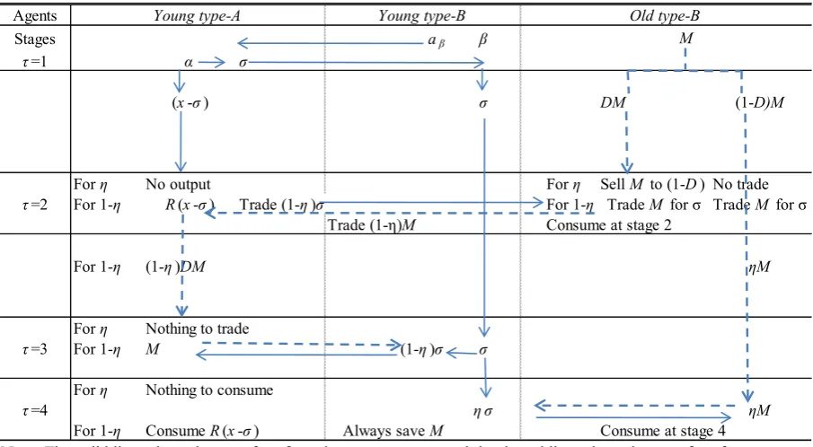
Figure 1. Trading Patterns and optimal allocation in the absence of commitment

Thus, the amount of good α available in the fourth stage is ησ , which will be distributed among agents with positive money balances. Specifically, (1−D)η generation-(t–1) type-B agents bring (1−D)ηM units of money in total. In addition, (1−D)(1−η) generation-(t– 1) type-B agents bring DηM units of money in total.

Those who choose to participate incur cost ε. Those who choose not to participate in exchange do not incur cost ε and leave the meeting with autarky.

4.2. Ex ante Steady-State Social Welfare and Constraints Figure 1 summarizes the trading patterns within a period, as explained in the previous sections. In the first column, we show the stages of trading within a period. In the remaining three columns, we report the trade made by the three types of agents: a young type-A agent, a young type-B agent, and an old type-B agent. In these columns, the solid lines show the transfer of goods among agents, and the dotted lines show the transfer of money balances among agents. We report the total amount of goods and money balances transferred among the agents or brought into the markets in each stage, and the details of the derivations are explained below.

We present the ex-ante steady-state social welfare and the relevant feasibility and incentive constraints. In what follows, we assume that ε = 0, following Mills and Reed [1].

We begin with the definition of aggregate ex ante welfare of type-A agents and type-B agents born in period t.

)]} ( ˆ [ ) 1 ( )] ( ˆ [ {

)]} ( ) ( ) ( [ ) 1 (

)] ( [ ){ 1 ( ] [

] ), 0 ( [

] ), ( ) ( [ ) 1 (

4 2

4 2

2

2 3

3 2

M b u D M

b u D

M b M t M b u D

M b u D b

u

a a u

a M a M a u U

B B

B

B B

A A

α α

α α

α

α β

β α

β α α

η

η η

η

⋅ − + ⋅

+

+ − ⋅

− +

⋅ − + +

⋅ +

+ −

=

(3)

The relevant constraints include feasibility constraints and incentive constraints in each stage imposed because of the lack of full information and commitment.

In the first stage, we have two feasibility constraints for the allocation of good α between two technologies and the allocation of good β between the generation-t type-A agents and the generation-t type-B agents:

x ≤

σ (4)

y b

aβ + β ≤ (5)

In the first stage, there are also two participation constraints for each type of agent, indicating that the expected value of participating in trade is at least as good as autarky for a type-A agent and for a type-b agent respectively.

] 0 , 0 [ ] 0 , [ ) 1 (

] ), 0 ( [

] ), ( ) ( [ ) 1 (

3

3 2

A A

A A

u Rx

u a a u

a M a M a u

⋅ + −

≥ ⋅ +

+ −

η η

η η

β α

β α α

(6) Agents

Stages aβ β

τ=1 α σ

(x-σ) σ DM (1-D)M

For η No output For η Sell M to (1-D) No trade

τ=2 For 1-η R(x-σ) Trade (1-η)σ For 1-η Trade M for σ Trade M for σ Trade (1-η)M Consume at stage 2

For 1-η (1-η)DM ηM

For η Nothing to trade

τ=3 For 1-η M (1-η)σ σ

For η Nothing to consume

τ=4 η σ ηM

For 1-η Consume R(x-σ) Always save M Consume at stage 4

Note: The solid lines show the transfer of goods among agents, and the dotted lines show the transfer of money balances among agents.

Young type-A Young type-B Old type-B

] 0 [ ] [ )]} ( ˆ [ ) 1 ( )] ( ˆ [ { )]} ( ) ( ) ( [ ) 1 ( )] ( [ ){ 1 ( ] [ 4 2 4 2 2 2 B B B B B B B u y u M b u D M b u D M b M t M b u D M b u D b u + ≥ ⋅ − + ⋅ + + − ⋅ − + ⋅ − + α α α α α α β η η (7)

The second-stage feasibility constraints state that agents cannot leave with more of good α than is available in that stage. For the 1–η meetings, in which there is a positive return from the risky investment technology, the available amount of good α is the realized return from the investment technology, R(x−σ). Because we expect that good α will be distributed to D generation-(t–1) type-B agents with M units of money, the feasibility constraint is:

) ( ) ( )

(_{x a}2 _{M b}2 _M

R −σ ≥ α + α (8)

For the η meetings in which there is zero output from the risky technology, there is no exchange of goods. The type-A agent will leave the market without obtaining money balances, and for the generation-(t–1) type-B agent, we have two additional feasibility constraints for the resale market of the collateral goods, equations (1) and (2).

In the second stage, there are participation constraints for type-A agents. A type-A agent’s utility of participating in trade should be greater than his utility of holding the realized return:

]

),

(

[

]

),

(

)

(

[

2 3

β β α α

σ

a

x

R

u

a

M

a

M

a

u

A A

−

≥

+

or simply: ) ( ) ( ) ( 3 2 _σ α

α M +a M ≥R x−

a (9)

If the type-A agent agrees to trade, he keeps

a

α2

(

M

)

of

good α and can use money to acquire

a

α3

(

M

)

in the third

stage. If he does not agree to trade, he has no money balances to acquire any of good α in the third stage but keeps all of his good α in the second stage.

In the second stage, there are also the participation constraints for the type-B agents as follows.

For (1–η)(1–D) type-B agents, they compare their utility of consumption in the second stage and in the fourth stage, and choose to trade in both the second and fourth stages, rather than trade only in the second stage, or trade only in the fourth stage as η (1–D) type-B agents who meet unproductive agents do:

)] 0 ( ) ( [ )] ( ) ( ) ( [ 4 2 4 2 2 α α α α α b M b u M b M t M b u B B + ≥ + − (10) )] ( ˆ [ )] ( ) ( ) (

[_b2 _{M t}2 _{M b}4 _{M u b}4 _M

uB B

α α

α

α − + ≥ (11)

For η(1–D) type-B agents, there is no reason to trade with unproductive type-A agents, and they wait to consume until the fourth stage. For the remaining D type-B agents, there is no alternative to consuming in the second stage, and thus the incentive constraint, equations (10) and (11), will not

apply to them. Note that in Mills and Reed [1], all type-B agents who consume in the second stage compare their utility of consumption in the second stage with that in the fourth stage, and the counterpart of equation (10) becomes

)] ( [ )] 0 ( ) (

[_b2 _{M b}4 _{u b}4 _M

uB B

α α

α + ≥ .

In the third stage, the generation-t type-A agents and the generation-t type-B agents who were matched in the first stage are reunited. The type-A agents have either zero or

M

units of money. The type-B agents are distinguished by whether or not they have σ units of good α. The mechanism suggests that:

0 ) 0 ( 3 ₌ α

a (12)

And

σ

α3(M)=

a (13)

In equation (12),

a

α3

(

0

)

=

0

comes from a lack of

commitment and an absence of public records of past transactions. If

a

α3

(

0

)

>

0

, a type-B agent would have to

give some good α to type-A agents for nothing. The type-B agent has an option to obtain money in the fourth stage by refusing to trade in the third stage and by keeping his collateral to sell in the fourth stage. Equation (12) shows the insurance role of collateral, which is a better trade for the type-B agent. Equation (13) is feasible if all the money balances held by the type-A agents are traded for goods held by the type-B agents. From the perspective of the type-A agents, this is the last opportunity to obtain goods, and thus the type-A agents are willing to trade all of their money balances. From the perspective of the type-B agents, they are happy to fulfill their promise to give the collateral back to the type-A agents and to obtain money balances. Hence, equation (13) is feasible and incentive compatible.

In the fourth stage, all of the remaining good α is transferred from the generation-t type-B agents to the (1–D) generation-(t–1) type-B agents. The amount of good α available is that which remains after the generation-t type-B agents transfer to the generation-t type-A agents in the third stage. In the third stage, generation-t type-B agents transfer to generation-t type-A agents (1−η)σ units of good α. Thus, the amount of good α available in the fourth stage is ησ, which will be distributed among agents with positive money balances. Specifically, (1−D)η _generation-(t–1) type-B agents bring (1−D)ηM units of money in total. In addition, (1−D)(1−η) generation-(t–1) type-B agents bring DηM units of money in total. Therefore, the total amount of money,ηM , will be exchanged for ησ units of good α. Remember that the mechanism suggests that:

0 ) 0 ( 4 ₌ α

b (14)

The feasibility constraint is:

ησ η

η − ⋅ α + − ⋅ α ≤

− )(1 ) ( ) (1 ) ˆ ( ) 1

The participation constraints for those with money and those with good α are satisfied. For the generation-(t–1) agents, it is the last chance for them to spend money to obtain good α for consumption. For the generation-t agents, it is the last chance for them to acquire money to prepare for their consumption of good α in period t+1.

4.3. The Optimal Allocation in the Absence of Commitment

The optimal allocation in the absence of commitment is a list: {σ, aβ, aα2(M), ( )

3 _M

aα ,aα3(0),

b

β ,bα2(M),

b

α4

(

0

),

bα4(M),

), (

2 _M

tα bˆα2(M),bˆα4(M)}, which maximizes (3) subject to (1), (2), and (4) through (15). To solve this problem, we set up the Lagrangian (16).

])} 0 [ ] [ ( )]} ( ˆ [ ) 1( )] ( ˆ [ { )]} ( ) ( ) ( [ ) 1( )] ( [ ){ 1( ] [ { ˆ ]} 0, 0 [ ] 0, [ ) 1( ] ,0 [ ] ), ( ) ( [ ) 1 {( )] ( ˆ ) ( ) ( ) ( [ ˆ )] 0 ( ) ( ) ( ) ( ) ( [ ˆ )] ( ) ( ) ( [ )] ( ˆ ) 1( ) ( ) 1 )( 1( [ ˆ )] ( ˆ ) ( ) 1 )( 1 [( ˆ )] ( ) ( [ ˆ )] ( ) ( ) ( [ ˆ ) ( )]} ( ˆ [ ) 1( )] ( ˆ [ { )]} ( ) ( ) ( [ ) 1( )] ( [ ){ 1( ] [ ] ), 0 ( [ ] , ) ( [ ) 1( 4 2 4 2 2 2 4 3 2 3 4 4 2 2 22 4 2 4 2 2 21 3 2 1 4 4 3 2 2 22 2 2 21 2 2 2 1 4 2 4 2 2 2 3 2 B B B B B B B A A A A B B B B B A A u y u M b u D M b u D M b M t M b u D M b u D b u u Rx u a u a M a M a u M b M b M t M b b M b M b M t M b x R M a M a M b D M b D M b D M t D M t M b M b M a x R b a y M b u D M b u D M b M t M b u D M b u D b u a a u a M a u L + − ⋅ − + ⋅ + + − ⋅ − + ⋅ − + + ⋅ − − − ⋅ + + − + − + − + − − + − + − − + + − − − − − + − − − + − + − − − + − − +                     ⋅ − + ⋅ + + − ⋅ − + ⋅ − + + ⋅ + + − = α α α α α α β β β α α α α α α α α α α α α α α α α α α α α α β β α α α α α α β β α β α η η γ η η η η γ γ γ σ γ η η ση λ η η λ λ σ λ λ η η η σ η (16)

To solve this problem, we set up the Lagrangian (16). The λ multipliers are associated with the remaining feasibility constraints, and the γ multipliers are associated with the participation constraints. All of the λ multipliers should be positive; otherwise, resources would be wasted.

4.4. Properties of the Optimal Allocation in the Absence of Commitment

We examine the properties of the optimal allocation in the absence of commitment. Result 1 summarizes the

consumption of type-B agents in the fourth stage.

Result 1: σ σ

η η

σ α

α = = _{− −} >

) 1 )( 1 ( ) ( , ) (

ˆ4 4

D D M b M b _.

Proof: As the feasibility constraint equation (15) binds, we have:

ησ η

η α + − α =

−

− )(1 ) ( ) (1 ) ˆ ( )

1

( _{D b}4 _{M D b}4 _M

Note that each (1–D)η type-B agent has M units of money while each (1–D)(1–η) type-B agent has {Dη /(1– D)(1–η)}M units of money, and goods will be allocated depending on their money balances. Hence,

σ σ

η η

σ α

α4(M)= D /{(1−D)(1− )}> ,bˆ4(M)=

b .

Result 2 summarizes the consumption of type-B agents in the second stage.

Result 2: σ σ

η η σ α α < − − = = D D M b M

b2( ) ,ˆ2( ) (1 )(1 )

. Proof: As equations (8), (9), and (13) hold with equality,

) ( )

( 2

3 _{M b M}

aα α

σ = = . As the feasibility constraint equations (1) and (2) bind, we have:

) ( ˆ ) ( ) 1 )( 1

( _{D b}2 _{M D b}2 _M

α

α η

η =

− −

Hence, bˆ_α2(M)₌σ(1₋D)(1₋η)/Dη_{. Taken together, we} obtain the following proposition:

Proposition 1: σ η η σ σ η η α α α α D D M b M b M b D D M b ) 1 )( 1( ) ( ˆ ) ( ˆ ) ( ) 1 )( 1( ) ( 2 4 2 4 − − = > = = > − − =

under our assumption that ηD > (1–η)(1–D).

Note that equation (10) is satisfied because )

( )

( 2

4 _{M b M}

bα > α and equation (11) is also satisfied because )

( ˆ )

( 4

4 _{M b M}

bα > α .

Proposition 1 comes from the fact that the late-departing type-B agents who meet productive type-A agents in the second stage are happy to consume at the fourth stage, rather than at the second stage. Otherwise, these agents will not offer goods for money submitted by the early-departing type-B agents who meet unproductive type-A agents.

Result 3 summarizes the level of consumption for a type-A agent.

Result 3: aα3(M)=σ ,aα2(M)=R(x−σ)−σ.

Now, we show that our model includes the optimal allocation in the absence of commitment studied by Mills and Reed [1] as a special case.

Result 4: When we set D = 0 and _t2(_M)₌0

α , the optimal

allocation obtained from equation (16) is the same as those obtained by Mills and Reed [1], which shows

σ

α α( )= ( )=

ˆ4 _{M b}2 _M

b .

Proof: As D=0, Result 1 shows _b4(_M)₌0

α . Note that

equation (15) holds with equality and by letting D=0 and 0

) (

4 _{M =}

equation (11), and we obtain bα2(M)≥bˆα4(M)=σ.

Now, note that equation (8) holds with equality, hence )

( ) ( )

(_{x a}2 _{M b}2 _M

R −σ = α + α . Insert this result into equation

(9) to yield _a2(_M) _a3(_M) _R(_x ) _a2(_M) _b2(_M)

α α α

α + ≥ −σ = + , thus

) ( )

( 2

3 _{M b M}

aα ≥ α . With equation (13), this expression means

that _b2(_M)

α

σ≥ . Therefore, combined with the result that

σ

α α2(M)≥bˆ4(M)=

b in the previous paragraph, we obtain σ

α2(M)=

b and bˆα4(M)=σ . Note that the resource allocation for a type-A agent in our model is the same as that of Mills and Reed [1].

5. Policies to Achieve Better Resource

Allocation

Proposition 1 shows that a taste shock regarding the timing of consumption when old will affect the ex-ante utility of type-B agents. The early-departing ηD old type-B agents, who meet unproductive young type-A agents in the second stage, will consume less of good α compared with the rest of the old type-B agents. The late-departing (1-η)(1-D) old type-B agents, who meet productive young type-A agents in the second stage, will consume more good α compared with the rest of the old type-B agents. We could improve the ex-ante utility of type-B agents if we had some policy tool to achieve

σ

α α

α

α( )= ( )= ˆ ( )= ( )= ˆ2 _{M b}2 _{M b}4 _{M b}4 _M

b .

In this section, we examine whether it is possible to improve the optimal resource allocations in the absence of commitment. One may think that the situation of the early-departing ηD old type-B agents is similar to that of early-departing old creditors in Freeman [13], who are forced to liquidate their loans below par value in the lending market under a liquidity constraint and cannot consume the same amount of goods as the late-departing creditors do. Remember that Mills and Reed [1] examine financial arrangements in the absence of commitment, with no public record of agents’ trading histories, and thus no institutional setup. From now on, we allow minimum deviation from the assumptions made by Mills and Reed [1], and examine whether an additional institutional setup might lead to a better resource allocation. In particular, we assume further that there is an agent called central bank that can implement the policy to achieve the desired resource allocation

σ

α α

α

α( )= ( )= ˆ ( )= ( )= ˆ2 _{M b}2 _{M b}4 _{M b}4 _M

b . What kind of policy

tools should a central bank use to achieve the desired allocation? We consider both a nontraditional monetary policy and a traditional monetary policy in the spirit of Freeman [13].

5.1. Nontraditional Monetary Policy

Consider the following nontraditional monetary policy tool. Imagine a central bank keeps all of the collateral goods α on behalf of young type-B agents. The central bank identifies ηD unproductive young type-A agents at the beginning of the second stage, and the central bank proposes that ηD young type-B agents, who are going to trade with those ηD unproductive type-A agents in the third stage, trade σ units of their collateral good α for M units of fiat money. The central bank obtains ηDM units of money from ηD early-departing old type-B agents, who are pleased to consume σ units of collateral good αin exchange for fiat money to make these trades possible. The sales of collateral goods from ηD young type-B agents to ηD early-departing old type-B agents suggested by the central bank would be justified by the convention of the US repo market that gives cash lenders the right of rehypothecation.

From the perspective of ηD young type-B agents, they are indifferent between trading with the central bank at the second stage and selling their collateral at the fourth stage to obtain M units of fiat money. From the perspective of ηD early-departing old type-B agents, it would be better to trade with a central bank that gives them σ units of collateral good α in exchange for M units of fiat money, rather than to trade with (1-η)(1-D) late-departing old type-B agents who give them bˆα2(M)=σ(1−η)(1−D)/ηD<σ units of good α

in exchange for M units of fiat money. From the perspective of unproductive young type-A agents, they know that they cannot retrieve their collateral goods in the third stage given the negative productivity shock in the second stage, and thus they do not mind if the young type-B agents trade their collateral goods with the central bank. Therefore, those transactions are incentive compatible for all agents.

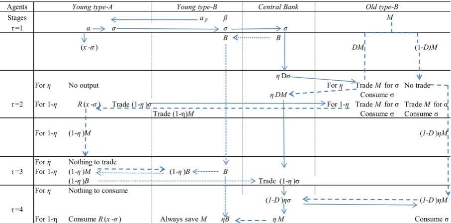
Because of the intervention by the central bank, as summarized in Figure 2, the amount of good α and units of money available in the second stage and in the fourth stage will be changed as described below.

First, the amount of good αavailable in the second stage is not (1−η)σ , but{1−(1−D)η}σ , because ηD young type-B agents sell their collateral to the central bank. The central bank sells ηDσ units of good α to the early-departing old type-B agents who meet the unproductive type-A agents, as the fourth column of Figure 2 shows. The amount of fiat money available in the second stage is the (1−η)M units that old type-B agents who meet the productive type-A agents bring and the DηM

units of money that the early-departing old type-B agents who meet the unproductive type-A agents bring, and thus

M D) } 1 ( 1

{ − − η in total. Hence, the monetary transaction in the second stage will trade M units of fiat money for σ

[image:11.595.78.532.78.302.2]

Figure 2. Trading patterns and optimal allocation with central bank intervention

Second, the amount of good α available in the fourth stage is not ησ, but (1−D)ησ , because ηD young type-B agents sell ηDσ units of good α to the central bank. The amount of fiat money available in the fourth stage is

M D)η 1

( − units that the (1−D)η old type-B agents bring. Hence, the (1−D)η old type-B agents will trade M units of fiat money for σ units of good α. In this way, the central bank intervention achieves the desired allocation

σ

α α

α

α( )= ( )= ˆ ( )= ( )= ˆ2 _{M b}2 _{M b}4 _{M b}4 _M

b .

Proposition 2: A central bank’s nontraditional monetary policy, which exchanges collateral goods held by ηD young type-B agents for fiat money held by ηD early-departing old type-B agents, will achieve a better resource allocation.

Proposition 2 shows that our nontraditional policy involves a transaction that is exactly opposite to that in the traditional Freeman [13] policy whereby the central bank should supply collateral goods, rather than fiat money. The central bank reallocates the available collateral goods from ηD young type-B agents, whose borrowers are unproductive agents, to ηD early-departing old type-B agents who are hit by a taste shock to their immediate consumption.

The central bank achieves welfare improvement first by collecting public information regarding the outcome of all investment projects based on bilateral contracts and then by encouraging quicker rehypothecation of the defaulting party’s collateral goods at the beginning of the second stage.

5.2. Traditional Monetary Policy À La Freeman [13] Our model is similar to that of Freeman [13], in which some of the lenders must depart from the lending market quickly and are forced to sell their loans below par value for

fiat money because the available amount of fiat money in the lending market is insufficient. However, the policy implication in our model is quite different from that of Freeman. In the case of Freeman [13], a central bank’s issue of additional fiat money in the resale market of IOUs resolves the lack of liquidity in that market and helps to achieve a better resource allocation. In our model, this traditional policy à la Freeman [13] cannot improve the resource allocation becauseadditional fiat money would not increase the type-A agents’ production of good αin time for the consumption by the lenders who are hit by a taste shock.

To make a central bank’s issue of additional fiat money effective, in the first stage, the central bank issues an additional M units of fiat money to purchase σ units of collateral goods from all the young type-B agents. Namely, the central bank must buy goods, rather than financial assets. In the second stage, the central bank sells ηDσ units of collateral goods to ηD early-departing old type-B agents, and obtains ηDM units of fiat money from those agents. In the third stage, the (1−

η

) productive young type-A agents get back (1−

η

)

σ

units of collateral goods from the central bank in exchange for the (1−

η

) M units of money. In the fourth stage, the central bank offers (1–D)η late-departing old type-B agents (1−D)

ησ

units of collateral goods in exchange for (1–D)ηM units of fiat money. At the end of the fourth stage, both the young type-B agents and the central bank have M units of fiat money. The central bank destroys the M units of fiat money in their possession.

After those operations, all of the other resource allocations are the same as the optimal resource allocations in the absence of commitment. However, the central bank must buy goods, rather than financial assets as traditional

Agents Central Bank

Stages aβ β

τ=1 α σ σ σ

B B

(x-σ) DM (1-D)M

ηDσ

For η No output For η Trade M for σ No trade

ηDM Consume σ

τ=2 For 1-η R(x-σ) Trade (1-η)σ For 1-η Trade M for σ Trade M for α

Trade (1-η)M Consume σ Consume σ

For 1-η (1-η)M (1-D)ηM

For η Nothing to trade

τ=3 For 1-η (1-η)M (1-η)B B

(1-η)B Trade(1-η)σ

For η Nothing to consume

(1-D)ησ (1-D)ηM

τ=4

For 1-η Consume R(x-σ) Always save M ηB ηM Consume σ

Note: The solid lines show the transfer of goods among agents, dotted lines show the transfer of bond among agents, and the dashed lines show the transfer of money balances among agents.

monetary policy à la Freeman [13] assumes.

6. Conclusions

In this paper, we show that a central bank could improve the allocation of resources by delivering the defaulting party’s collateral goods to those who consume the most quickly.

To show this point, we extend Mills and Reed [1] by examining the effects of shocks to lenders’ consumption in the second period of their lives. Thanks to the role of collateral as insurance against a borrower’s default, lenders have the same money balances at the beginning of the second period of their lives, consistent with Mills and Reed [1]. However, unlike Mills and Reed [1], they may not enjoy the same level of consumption in the second period of their lives if they are hit by shocks to the lenders’ consumption, and thus their expected utilities will decrease.

Specifically, suppose that some lenders are hit by a taste shock at the beginning of the second period of their lives that forces them to consume within an early stage of the second period of their lives. Suppose further that the amount of goods available within an early stage of the second period of their lives is not enough to meet the demand for goods from the lenders hit by a taste shock, while more goods are available in the later stages of the second period of their lives on the resale market for collateral goods. In that case, the level of consumption in the second period of their lives could vary depending on the timing of consumption, even though they are insured against their borrowers’ default in the first period of their lives. We show that a central bank could deliver the defaulting party’s collateral goods to those who consume the most quickly, could make the consumption of lenders constant and independent of the timing of transactions in the goods market, and could achieve better resource allocation by using nontraditional monetary policy.

It is true that other institutional setups, such as a private CCP or public ledger of all transactions of collateral goods, would achieve better resource allocation as nontraditional monetary policy tools do. However, the division of labor between institutions is one of the issues beyond the scope of this paper because the model in this paper assumes that there is no public record keeping of agent histories and no repeated relationships between a borrower and a lender. These assumption prevent us from making a particular policy recommendation for some economic institutions based on the model in this paper.

Acknowledgements

The author would like to thank Will Roberds, Hector Perez Saiz, Florian Heider, Edoardo Rainone, Francisco Rivadeneyra, Marie Hoerova, Philipp Hartmann, James J. McAndrews, seminar participants at the ECB, Osaka

University and Hitotsubashi University, and participants of the International Conference on Payments and Settlement hosted by Deutsche Bundesbank, Singapore Economic Review Conference 2015, and the Asian Meeting of the Econometric Society 2016 for their helpful comments on this draft. The author also would like thank David Mills, Charles M. Kahn, and James Chapman for their helpful suggestions on my related work on “Default Risks and Collateral in the Absence of Commitment in a Two-country Model.” This work was supported by JSPS Kaken Grant Number 268850083 and a research fund from Tokyo Center for Economic Research.

REFERENCES

[1] D. C. Jr. Mills and R. R. Reed, “Default Risk and Collateral in the Absence of Commitment,” 2012, The Selected Works of David C Mills Jr, Online available from http://works.bepress.com/davidcmills/1

[2] Lacker J. M., Collateralized Debt as the Optimal Contract, Review of Economic Dynamics 4(4), 2001, pp. 842–859. [3] Rampinib, A. A., Default and Aggregate Income, Journal of

Economic Theory 122(2), 2005, pp. 225–253.

[4] T. Kehoe, and D. K. Levine, Bankruptcy and Collateral in Debt Constrained Markets, in Macroeconomics in the Small and the Large, Ed. Roger E. A. Farmer, 2008, Edward Elgar. [5] Shi S., Credit and Money in a Search Model with Divisible

Commodities, Review of Economic Studies 63(4), 1996, pp. 627–652.

[6] Mills, D. C. Jr., Mechanism Design and the Role of Enforcement in Freeman’s model of Payments, Review of Economic Dynamics 7(1), 2004, pp. 219–236.

[7] Mills, D. C. Jr., Alternative Central Bank Credit Policies for Liquidity Provision in a Model of Payments, Journal of Monetary Economics 53(7), 2006, pp. 1593–1611.

[8] L. Ferraris, M. Watanabe. Collateral Secured Loans in a Monetary Economy, Journal of Economic Theory 143(1), 2008, pp. 405–424.

[9] K. D. Garbade, F. M. Keane, L. Logan, A. Stokes, J. Wolgemuth. The Introduction of the TMPG Fails Charge for U.S. Treasury Securities, FRBNY Economic Policy Review, October 2010, pp. 45–71.

[10] A. Copeland, I. Selig. Don’t Be Late! The Importance of Timely Settlement of Tri-Party Repo Contracts, Liberty Street Economics,

October 20, 2014. Online available fromhttp://libertystreetec onomics.newyorkfed.org/2014/10/dont-be-late-the-importan ce-of-timely-settlement-of-tri-party-repo-contracts.html#.VE 3NefmsXUV

[11] M. Fleming, F. Keane, A. Martin, M. McMorrow. Measuring Settlement Fails, Liberty Street Economics, September 19, 2014a. Online available from

ring-settlement-fails.html#.VB4PWu9xmZM

[12] M. Fleming, F. Keane, A. Martin, M. McMorrow. What Explains the June Spike in Treasury Settlement Fails? Liberty Street

Economics, September 19, 2014b. Online available from http ://libertystreeteconomics.newyorkfed.org/2014/09/what-expl ains-the-june-spike-in-treasury-settlement-fails.html

[13] Freeman S, The Payments System, Liquidity, and Rediscounting, American Economic Review 86 (5), 1996, pp.

1126–1138.

[14] Monnet C., Let’s Make It Clear: How Central Counterparties Save(d) the Day, Business Review, Q1, Federal Reserve Bank of Philadelphia, 2010, pp.1-10.

[15] Green E. J., Money and Debt in the Structure of Payments, Monetary and Economic Studies 15 (1), 1997, pp. 63–87. [16] C. Monnet, T. Nellen, “The Collateral Costs of Clearing,”