Forecasting load demand using ERACS

Forecasting Load Demand Using ERACS

1

Shamsul Aizam Zulkifli,

Md Zarafi Ahmad,

Rohaiza Hamdan,

Andrea Luxman

Abstract - The electric power demand of Universiti Tun Hussein Onn Malaysia (UTHM) has steadily increased in the past five years. This trend is certain to continue in future. Due to this matter theelectricity load forecasting is thus an important topic, since accurate forecasts can avoid wasted energy and to prevent system failure. It is very important for the university to have advance knowledge of electrical load usage, to ensure the load is stable and to minimize the usage which contributes to decreased the cost of operation. This paper is to predict of maximum load in UTHM up to year 2016 with an interval of three years in between discussed using a statistical method and ERACS software to calculate the loadflow and followed by derivation of forecasting equations using MATLAB software. This method of forecasting is categorised as long term load forecasting.

Index terms: Forecasting, ERACS, MATLAB, UTHM

I. INTRODUCTION

The electric power demand of Universiti Tun Hussein Onn Malaysia (UTHM) has steadily increased in the past seven years. This trend is certain to continue in future. The electrical load is the power that an electrical utility needs to supply in order to meet the demands of its customers. Electricity load forecasting is thus an important topic, since accurate forecasts can avoid wasting energy and prevent system failure [1]. It is no need to generate power above a certain predictable level and the latter when normal operation is unable to withstand a predictable heavy load. For example, short-term planning of electricity load generation allows the determination of which devices shall operate and which shall not in a given period, in order to achieve the demanded load at the lowest cost. It also helps to schedule generator maintenance routines. The system operator is responsible for the scheduling and aims foremost at balancing power production and demand. After this requirement is satisfied, it aims at minimizing production costs, including those of starting and stopping power generating devices, taking into account technical restrictions of electricity centrals. Finally, there must always be a production surplus, so that local failures do not affect dramatically the whole system [2].

1_{Shamsul Aizam Zulkifli is with Universiti Tun Hussein Onn Malaysia,}

Batu Pahat, Johor, Malaysia. He can be reached at [email protected]

2_{Md Zarafi Ahmad is with Universiti Tun Hussein Onn Malaysia, Batu}

Pahat, Johor, Malaysia. He can be reached at [email protected]

3_{Rohaiza Hamdan is with Universiti Tun Hussein Onn Malaysia, Batu}

Pahat, Johor, Malaysia. She can be reached at [email protected]

4_{Andrea Luxman can be reached at [email protected].}

How to estimate the future load with the historical data has remained a difficulty up to now. With the recent development of new mathematical, data mining and artificial intelligence tools, it is potentially possible to improve the forecasting result

There are various methods to produce such forecasts. A method may be said to be good if it at most times is able to predict the power load with good precision [3]. In this paper, a proposal of a long-term load forecasting method, using ERACS Software by ERA Technologies is done. It has also been found that not many authors have done much research on long term power load demand forecast as compared to short term load forecast.

II. DEVELOPMENT OF UTHM DISTRIBUTION NETWORK

The diagram of entire power system network of UTHM is obtained from Property and Development Department. The generator, grid, and busbar ratings are based on the labeling on the drawing itself.

Along with the diagram, load real power and reactive power readings which are in kWh and kVArh respectively for each electric substation is also collected. The load power reading is based on the TNB tariff bill which states the amount of real and reactive power consumed per electric substation. The data collected is for the month of December 2007 and is taken as the reference data for the entire network. Using this data, the reactive power, kVAr and real power, kW for each load is calculated using average load demand formula. In the case where reactive power is not stated, trigonometric calculation of the power triangle whereby the power factor is set at 0.85 is used to determine the reactive power.

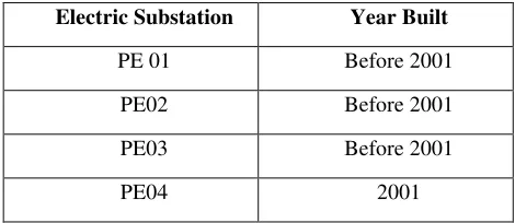
Another set of important data collected was the year that each electric substation was built. This data is used to calculate loadflow for four specific years with an interval of three years between each year. Below is the table of when each electric substation was built.

TABLE I YEAR THAT EACH ELECTRIC SUBSTATION WAS BUILT

Electric Substation Year Built

PE 01 Before 2001

PE02 Before 2001

PE03 Before 2001

PE04 2001

PE05 2001

PE06 2004

PE07 2004

PE08 2005

PE09 2005

PE10 2005

PE11 2005

PE12 2007

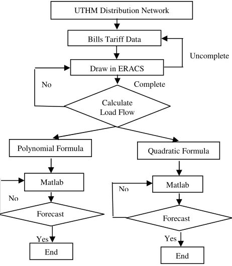
The power system network is drawn using a power system simulation software known as ERACS. Four separate networks are drawn according to the four predetermined years which are before 2001, 2001, 2004 and 2007, all of which have an interval of three years between them. Data collected and calculated are keyed into the software for it to perform loadflow study through simulation. Loadflow simulation in ERACS is used to determine six types of power flows in the network which are reactive power generated, real power generated, real power at load, reactive power at load, real power loss and reactive power loss. Once loadflow simulation is performed, the results for all four sets of networks are recorded and are used in the analysis section where forecasting of future load demand is carried out. Fig. 1 shows the process flows in forecasting the network using ERACS and MATLAB.

Fig. 1: Process methodology

III. RESULTS

A. UTHM Power System Network

The load flow of the UTHM power system network is studied from before 2001 to 2007 in intervals of three years, i.e, before 2001, 2001, 2004 and 2007. This data is then be used for the purpose of forecasting. There are two incoming power supplies which is the grid input and the synchronous generator. However only the grid inlet is used as the synchronous generator. The grid input is supplied by Tenaga Nasional Berhad (TNB). The voltage supplied through the grid is 11kV which is then connected to the main busbar. The main busbar connects the load of real and reactive power, in this case electric substations that supply electricity to the university buildings and infrastructures according different areas. In between each electric substation and the main busbar is a transformer that acts to step-down the input voltage of 11kV to 415V.

The loadflow summary of the network is obtained through the simulation using ERACS. Fig 2 shows the UTHM network.

Fig. 2: UTHM network in 2007 using ERACS

The total number of substations at present is 12. The increased in the number of substations is due to the expending of the university with more buildings and infrastructures having been added. The real power generated to the network increased to 12.162MW and the reactive power generated was 3.597MVAr. As a general from 2001 to 2007 loads data, the real power at load is 12.156MW and the reactive power at load is 3.489 MVAr. The real power loss is fluctuated until at 0.005MW for 2004 and 2007 due to none expenditure of the No

No

Bills Tariff Data

Uncomplete

Draw in ERACS

Calculate Load Flow

UTHM Distribution Network

Yes

No

Polynomial Formula

End

Yes Matlab

Quadratic Formula

End Complete

university buildings while the reactive power loss is 0.107MVAr, for the entire network until 2007.

B. Forecasting Results

The forecasted values are obtained by using two types of equations which are the linear polynomial line and quadratic polynomial line equations derived from MATLAB. This is done by the data been retable and analyzed. Although it would be ideal if the forecasted values would follow a linear trend, it is almost unlikely for that to happen. Hence, these two equations are used for the purpose of comparison. All the figures show the trend of data available when the distribution network has been analysis.

Fig. 3: Real power generated

Fig. 4: Reactive power generated

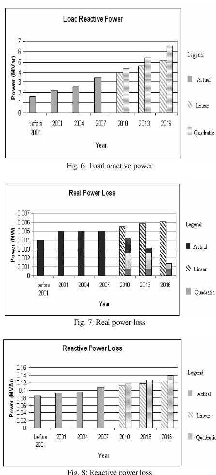
Fig. 5: Load real power

Fig. 6: Load reactive power

Fig. 7: Real power loss

Fig. 8: Reactive power loss

All the trends showing the increasing in reactive and power at both ends and the forecasting period for year 2010, 2013

and 2016 using linear and quadratic formula. In forecasting, an important aspect to be considered is the

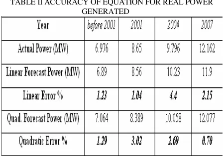
accuracy or precision of the values obtained using the forecast equation. Here, the actual values of before 2001, 2001, 2004 and 2007 are compared to the forecast values of the same years. The percentage of error is determined and based on the boundary of error, the most suitable type of equation to be used whether linear polynomial and quadratic polynomial is decided.

Percentage of Error = x100%

e ActualValu

lue ForecastVa e

ActualValu

   



 ₋₋₋₋

TABLE II ACCURACY OF EQUATION FOR REAL POWER GENERATED

Boundary of error for linear forecast is 1.04% to 4.4% while for boundary of error for quadratic forecast is 0.7% to 3.02%.

TABLE III ACCURACY OF EQUATION FOR REACTIVE POWER

Boundary of error for linear forecast is 1.86% to 7.73% and boundary of error for quadratic forecast is 1.07% to 5.08%.

TABLE IV ACCURACY OF EQUATION FOR LOAD REAL POWER

Boundary of error for linear forecast is 1.06% to 4.44% meanwhile boundary of error for quadratic forecast is 0.72% to 3.05%.

TABLE V ACCURACY OF EQUATION FOR LOAD REACTIVE POWER

Boundary of error for linear forecast is 2.57% to 7.92% with boundary of error for quadratic forecast is 1.24% to 5.87%

TABLE VI ACCURACY OF EQUATION FOR REAL POWER LOSS

.

Boundary of error for linear forecast is 2% to 8% and boundary of error for quadratic forecast is 1% to 3%.

TABLE VII ACCURACY OF EQUATION FOR REACTIVE POWER LOSS

Boundary of error for linear forecast is 1.04% to 4.4%and boundary of error for quadratic forecast is 0.7% to 3.02%

IV. CONCLUSION

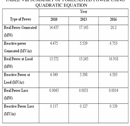
The techniques is to provide the local electrical utility company an estimated value of reactive and real power to be generated to UTHM so that there would be sufficient power supplied despite the university being continuously expanded over the coming nine years. It can also be used to avoid cases of overloading where too much of power is supplied and wasted causing unnecessary expenditure. At the same time, the forecasted value for the load consumption is useful for UTHM’s management so that they would have a rough idea as to the amount of real and reactive power that will be consumed and be able to plan for further expanding of the university available for forecasting the future trends in electricity demand in UTHM applications and at the same time plan financially the amount of money that would be spent on the cost of electricity. Table VIII shows the summary forecasted data that available for forecasting the future trends in electricity demand in UTHM applications that they would have a rough idea as to the amount of real and reactive power that will be consumed and be able to plan for further expand for the university.

TABLE VIII SUMMARY OF FORECASTED POWER USING QUADRATIC EQUATION

VII. REFERENCES

[1] J.Yang, “ Power System Short-term Load Forecasting.” Online thesis, Institute of Electrical Power Systems, Darmstadt University of Technology, November 2006.

[2] R.F. Engle, C. Mustafa, J. Rice, “Modeling Peak Electricity Demand.” Journal of Forecasting, Vol. 11, 1992. pp 241 – 251.

[3] R. Felix, “Electric Power Load Forecasting Using Periodic Piece-Wise Linear Models.” Online thesis, Institution of Mathematical Statistics, Technical University of Lund, March 2003.

[4] C. Jaipradidtham, Next Day Load Demand Forecasting of Future in Electrical Power Generation on Distribution Networks using Adaptive Neuro-Fuzzy Inference, Power and Energy Conference, 2006. PECon '06. 28-29 Nov. 2006 Page(s):64 – 67

[5] Chao-Ming Huang; Hong-Tzer Yang, “A time series approach to short term load forecasting through evolutionary programming structures”, Energy Management and Power Delivery, 1995. Proceedings of EMPD '95., Volume 2, 21-23 Nov. 1995

[6] Mandal, J.K.; Sinha, A.K, Artificial neural network based hourly load forecasting for decentralized load management, Energy Management and Power Delivery, 1995. Proceedings of EMPD '95., Volume 1, 21-23 Nov. 1995 Page(s):61 - 66 vol.1

[7] M.S. Kandil, S.M. El-Debeiky, N.E. Hasanien, “Long-Term Load

Forecasting For Fast Developing Utility Using A Knowledge-Based Expert.” IEEE Transaction Power Systems, Vol. 17, May 2002. pp. 491-496.

[8] K. Siwek, S. Osowski, “Short Term Load Forecasting In The Power

System Using Neural Networks.” IEEE Journal, 2000.

[9] A.G. Parlosl, E. Oufi, J. Muthusami, A.D. Patton, “Development Of An Intelligent Long-Term Electric Load Forecasting System.” IEEE Journal, 1996. pp. 288-292.

[10] A. Ku, “The Art of Forecasting Demand.” Global Energy Business Journal, March/April 2002. pp. 19-23.

[11] H.T.Yang, C.M. Huang, C.L. Huang, “Identification of ARMAX model

for short-term load forecasting, An evolutionary programming approach” IEEE Transactions on Power Systems, Vol.11, 1996. pp. 403 – 408

VII. BIOGRAPHIES

Shamsul Aizam Zulkifli obtained his B.Eng degree in Electrical & Electronic Engineering and Msc at University Putra Malaysia, Malaysia in 2003, 2006. Currently he is a lecturer and researcher in Universiti Tun Hussein Onn Malaysia. His interest areas are power quality problems, custom power devices and power system studies.

Md Zarafi bin Ahmad obtained his B.Eng degree in Electrical & Electronic Engineering and M Eng. at UiTM and UTM respectively. Currently he is a lecturer and researcher in Universiti Tun Hussein Onn Malaysia. His interest areas are power electronics and drives applications.

Rohaiza Hamdan obtained her B.Eng degree in Electrical & Electronic Engineering and M Eng. at UNITEN and UTM respectively. Currently she is a lecturer and researcher in Universiti Tun Hussein Onn Malaysia. Her interest areas are high voltage engineering and power system applicatios.