Framework and Analysis of Transit Scheduling using Multi- Size Vehicles

(1)

International Journal of Emerging Technology and Advanced Engineering

Website: www.ijetae.com (ISSN 2250-2459,ISO 9001:2008 Certified Journal, Volume 4, Issue 6, June 2014)

682

Framework and Analysis of Transit Scheduling using

Multi-Size Vehicles

Avishai (Avi) Ceder

1

Transportation Research Centre, Department of Civil and Environmental Engineering, University of Auckland, New Zealand, andCivil and Environmental Engineering Faculty, Technion – Israel Institute of technology

Abstract— This work addresses two transit

operations-planning activities: timetable development and vehicle-scheduling with different vehicle sizes and types. The work is a mixture between reviewed and new methodologies including some case studies. Alternative timetables are constructed with either even headways, but not necessarily even passenger loads or even average passenger loads, but not even headways. A method to construct timetables with the combination of both even-headway and even-load is developed for multi-size vehicles. A case study shows that the original passenger-load discrepancy from the desired load can be reduced from 38% to a discrepancy between 0% - 15% and at the same time preserving the time deviation from the determined even headway in the range of 0% - 7%. In addition a bi-objective approach is introduced to show how to make transit services more attractive by using two simultaneous objectives: minimizing the expected passenger waiting time and minimizing the discrepancy from a desired occupancy level on the vehicles. A case study of this bi-objective approach shows that the waiting time for passengers can be improved by more than 43% for the same level of empty-seat km. The vehicle-scheduling problem is based on given sets of trips and vehicle types arranged in decreasing order of vehicle cost using the deficit-function theory. Overall, prudent use of transit vehicles with different sizes can make the transit service more reliable and more economical.

Keywords— Multi-Vehicle Size, Public Transport,

Scheduling, Timetables, Transit.

I. INTRODUCTION

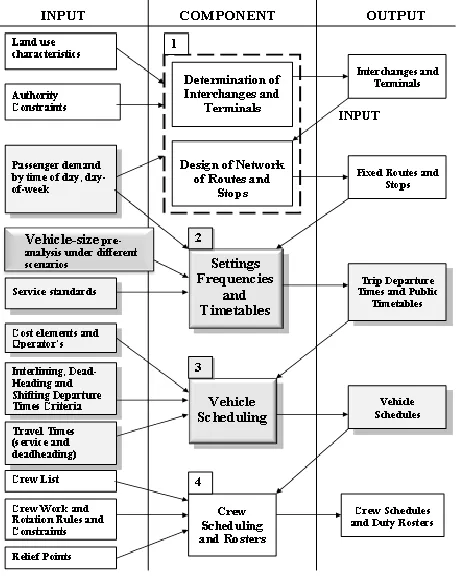
The public-transport (transit) operation planning process commonly includes four basic activities, usually performed in sequence: (1) network route design, (2) timetable development, (3) vehicle scheduling, and (4) crew scheduling [1]. Figure 1 shows the systematic decision sequence of these four planning activities including the new element of vehicle-size consideration. The output of each activity positioned higher in the sequence becomes an important input for lower-level decisions. Clearly the independence and orderliness ofthe separate activities exist onlyin the diagram; i.e., decisions made further down the sequence will have some effect on higher-level decisions.

It is desirable, therefore, that all four activities be planned simultaneously in order to exploit the system’s capability to the greatest extent and maximize the system’s productivity and efficiency. Occasionally the sequence in Figure 1 is repeated; the required feedback is incorporated over time. However since this planning process, especially for medium to large fleet sizes, is extremely cumbersome and complex, it requires separate treatment for each activity, with the outcome of one fed as an input to the next.

This work is three fold. First, it reviews different models to determine transit-vehicle size. Second, it focuses on timetable development with different, possibly available, vehicle sizes to improve the transit service. Third, it considers different vehicle types in the process of creating optimal vehicle schedules. The aim of public timetables is to meet general public transportation demand. This demand varies during the hours of the day, the days of the week, from one season to another, and even from one year to another. It reflects the business, industrial, cultural, educational, social, and recreational transportation needs of the community. Alternative timetables are determined on the basis of passenger counts, and they must comply with service-frequency constraints. The vehicle-scheduling activity in Figure 1 is aimed at creating chains of trips; each is referred to as a vehicle schedule according to given timetables. This chaining process is often called vehicle blocking (a block is a sequence of revenue and non-revenue activities for an individual vehicle). A transit trip can be planned either to transport passengers along its route or to make a deadheading trip in order to connect two service trips efficiently.

(2)

International Journal of Emerging Technology and Advanced Engineering

[image:2.612.57.285.140.428.2]

683

Figure 1. Framework of transit operational-planning process with emphasis on the themes of work

Commonly the consideration of vehicle size in transit-operations planning involves two considerations: first, determining the suitable or optimal vehicle size; second, choosing vehicles with different comfort levels, depending on trip characteristics. Certainly a multi-criteria effort may treat both considerations simultaneously, but this is seldom done in practice. The issue of what vehicle size/type to consider arises when purchasing a vehicle or a fleet of vehicles, an undertaking that is not performed frequently. The main purposes of this work are (a) to insert the variable of vehicle size in constructing efficient timetables with even headways, even loads and minimum waiting times, and (b) to address a minimum-cost vehicle-scheduling problem using graphical-based and math-programing approaches.

II. REVIEW ON TRANSIT SCHEDULING

This section covers concisely the literature of the two activities: timetable development and vehicle scheduling.

A. Timetabling

The problem of finding the best dispatching policy for transit vehicles on fixed routes has a direct impact on constructing timetables. This dispatching-policy problem, which has been dealt with quite extensively in the literature, can be categorized into four groups: (1st) models for an idealized transit system, (2nd) simulation models, (3rd) mathematical programming models, and (4th) data-based models.

The first group, idealized transit systems, was investigated by, for example, [2-4]. Newell [2] assumed a given passenger-arrival rate as a smooth function of time, with the objective of minimizing total passenger waiting time. De Palma and Lindsey [3] develop a method for designing an optimal timetable for a single line with only two stations. Wirasinghe [4] considered the average value of a unit waiting time per passenger (C1) and the cost of dispatching a vehicle (C2) to show that the passenger-arrival rate in Newell’s square root formula is multiplied by (C1/2C2).

In the second group, simulation models were studied by, for example, Adamski [5], and Dessouky et al. [6]. Adamski employed a simulation model for real–time dispatching control of transit vehicles while attempting to increase the reliability of service in terms of on-time performance. Dessouky et al. used a simulation analysis to show that the benefit of knowing the location of the bus was most significant when the bus was experiencing a significant delay.

In the third group, mathematical programming methods have been proposed, for example by Furth and Wilson [7], and Gallo and Di-Miele [8]. Furth and Wilson sought to maximize the net social benefit, consisting of ridership benefit and waiting-time saving, subject to constraints on total subsidy, fleet size, and passenger-load levels. Gallo and Di-Miele produced a model for the special case of dispatching buses from parking depots. Their model is based on the decomposition of generalized assignments and matching sub-problems. In the fourth and last group, the data-based models described in this work are based on Ceder [1,9].

B. Vehicle Scheduling

(3)

International Journal of Emerging Technology and Advanced Engineering

684 The number of feasible solutions to this problem is extremely high, especially in the case in which the vehicles are based in multiple depots. Much of the focus of the literature is, therefore, on computational issues.

Löbel [10] discussed the multiple-depot vehicle scheduling problem and its relaxation into a linear programming formulation that can be tackled using the branch-and-cut method. Freling et al. [11] discussed the case of single-depot with identical vehicles, concentrating on quasi-assignment formulations and auction algorithms. Huisman et al. [12] proposed a dynamic formulation of the multi-depot vehicle scheduling problem. The traditional, static vehicle scheduling problem assumes that travel times are a fixed input that enters the solution procedure only once; the dynamic formulation relaxes this assumption by solving a sequence of optimization problems for shorter periods.

Recent contributions noted are of Zak [13] who developed a multi-criteria optimization method for bus scheduling using two criteria from the passenger perspective and two – from the operator perspective with satisfactory results. In addition studies of integrated multi-depot vehicle and crew scheduling can be found by Borndorfer et al. [14], Gintner et al. [15] and Mesquita et al. [16] that use integer mathematical formulation, relaxation methods and heuristics to overcome the basic NP-Hard problem. Other related recent studies search for relief opportunities to approach optimal crew scheduling at transit stops where the drivers can be switched. Such studies are presented by Kwan and Kwan [17] and Laplagne et al [18].

III. BACKGROUND ON EVEN-HEADWAY AND EVEN-LOAD

TIMETABLES

Procedures to construct alternative timetables appear in Ceder [1,9]. The automated timetables are constructed with either even headways, but not necessarily even loads on board individual vehicles at the peak-load section, or even average passenger loads on board individual vehicles, but not even headways. Average even loads on individual vehicles can be approached by relaxing the evenly spaced headways pattern (through a rearrangement of departure times).

A. Even-Headway Timetables with Smooth Transitions

One characteristic of existing timetables is the repetition of the same headway in each time period. However, a problem facing the scheduler in creating these timetables is how to set departure times in the transition segments between adjacent time periods.

A common headway smoothing rule in the transition between time periods is to use an average headway. Many transit agencies employ this simple rule, but it may be shown that it can result in either undesirable overcrowding or underutilization.

For example, consider two time periods, 07:00-08:00 and 08:00-09:00, in which the first vehicle is predetermined to depart at 07:00. In the first time period, the desired occupancy (desired load) is 50 passengers, and in the second 55 passengers. The observed maximum demand to be considered in these periods is 148 and 192 passengers, respectively. These observed loads at a single point are based on the uniform passenger-arrival-rate assumption. The determined frequencies are 148/50 = 2.96 vehicles and 192/55 = 3.49 vehicles for the two respective periods, and their associated rounded headways are 20 and 17 minutes, respectively. One of the issues facing a scheduler is to determine the transition headway so as to avoid overcrowding and be efficient at the same time. The following principle and proposition pave the way to solve this issue [1,9].

Principle 1: Establish a curve representing the cumulative (non-integer) frequency determined versus time. Move horizontally for each departure until intersecting the cumulative curve, and then vertically; this will result in the required departure time.

Proposition 1: Principle 1 provides the required evenly spaced headways with a transition load approaching the

average desired occupancies of doj and do(j+1) for two consecutive time periods, j and j+1.

(4)

International Journal of Emerging Technology and Advanced Engineering

[image:4.612.55.286.150.403.2]

685

Figure 2. Determination of evenly spaced headways B. Even-Load Timetables

The results of Procedure 1 starts with the 7:20 and 7:40 departures for j = 1. The frequency required, based on the hourly Max load point, is 2.96 for j = 1. This frequency aimed at 50 passengers per vehicle while considering the entire hourly max demand. Given are the observed passenger loads at the Max load point between 7:00-8:00, that is, 65 (of 7:15 departure), 35 (of 7:45 departure). However, the assumption of uniform passenger arrival rate, between the observed departures, results in 65/15 = 4.3 passengers/minute between 7:00 and 7:15 and 35/30 = 1.2 pass/min between 7:15 and 7:45. Therefore, the 7:20 departure (by Procedure 1) may result in 65 + 1.2 x 5 = 71 passengers; significantly above the desired 50 passengers. In order to avoid this imbalanced situation the following principle is exploited.

Principle 2: Construct a curve representing the cumulative loads observed on individual vehicles at the hourly Max load points. Move horizontally per each doj for all j, until intersecting the cumulative-load curve, and then vertically; this results in the required departure times.

Proposition 2:Principle 2 results in departure times such that the average Max load on individual vehicles at the hourly jth Max load point approaches the desired occupancy doj.

Proof: Figure 3 illustrates Principle 2 for the example used. The derived departure times are unevenly spaced to obtain even loads at points at the Max load points. These even loads are constructed on the accumulative curve to approach d1 and d2 for j = 1, j = 2, respectively.

Assuming uniform passenger arrival rate between each two observed departures shows that the load of the 7:45 departure, for example, is comprised of the arrival rate between 7:12 and 7:15 (65/15 = 4.3) and the rate between 7:15 and 7:45 (35/30 = 1.2). Thus, 4.3 x 3 + 1.2 x 30 = 49 which is approaching d1 = 50. Moreover, in the transition between j = 1 and j = 2, the value of d2 = 55 is considered because the resultant departure is after 8:00. Given are the observed passenger loads at the Max load point between 8:00-9:00, that is, 25 (of 8:10 departure), 94 (of 8:30 departure), and 88 (of 8:50 departure). Therefore, the load of the vehicle departing on 8:16 at its hourly max load point, is comprised of (25/25) x 25 + (94/20) x 6= 53.2 which is approaching d2 = 55. The exact value of d2 can be obtained only for departures with non-integer minutes. This completes the proof-by-construction of Proposition 2.

[image:4.612.328.557.436.679.2]

(5)

International Journal of Emerging Technology and Advanced Engineering

686

IV. COMBINING EVEN-LOAD AND EVEN-HEADWAY

TIMETABLES USING DIFFERENT VEHICLE SIZES

Currently and commonly, as is known, bus timetables are based on even-headway departures. The even-headway feature for a given time period reduces the flexibility of the scheduler to accommodate fluctuations in demand within this period. This lack of flexibility may result in undesirable operational scenarios such as overcrowding or vehicles running almost empty. Uneven loads lead to either passenger discomfort, in case of overcrowding, or uneconomical and energy inefficient operation of the vehicles in the latter case [19,20]. However, the even-load timetables can lead to long and exceedingly irregular headways and thus to increase the waiting times for passengers arrived randomly. To overcome the disadvantages of both approaches (even-headway and even-load) this section aims at making the transit service more attractive by creating timetables using different types and sizes of vehicles to achieve even headways with minimum uneven loads at the max-load point(s). The quality of the timetables is based on two criteria: load discrepancy on the vehicles from a desirable load, and time discrepancy from a desirable headway.

The load discrepancy criterion serves as an indicator of how the actual max-point load on the vehicles deviates from a desired occupancy level (e.g., number of seats) including a buffer for demand fluctuations. The time discrepancy criterion provides information about how evenly the headways are spaced in the final timetable based on the calculation of average waiting time per passenger. Two approaches are presented using different (could be perceived as available) vehicle sizes; the first is heuristic-based to attain both even load and even headway, and the second is optimization-based to attain minimum waiting time and even load.

A. Heuristic Approach

As is shown in Ceder [1] the expected waiting time for randomly arriving passengers, Wt, can be calculated as follows:

( _{( )} ) (1)

This formula shows that the expected waiting time is minimal for even headways. For evenly distributed arrivals the best headway for a single size of vehicle can be easily found by dividing the total number of passengers observed at the Max load point by the desired passenger load.

However, in reality, arrivals show fluctuations and are far from being evenly distributed. Consequently the proposed methodology uses a heuristic procedure to determine the optimal headway for a fluctuated demand using different vehicle sizes. For convenience the use of seat capacity determines the size of the vehicle; this seat capacity term is compared with the desired passenger load (desired occupancy or load factor).

In each step, of the heuristic procedure, vehicles are assigned departure times based on an even-headway timetable such that the Max load demand is satisfied. Having different vehicle sizes available, the choice of vehicle is sometimes ambiguous. Therefore, three main strategies are considered:

Strategy C1: Minimizing the size of the vehicle by assigning the largest vehicle size amongst all available vehicles such that its seat capacity is less than, or equal to, the average observed (hence expected) passenger load, That is, for a departure at time t with an expected load of

L(t), ( ) where Skand Sk-1are two following

available vehicle sizes, and the assigned vehicle is the one with the seat capacity of Sk-1. This may imply overcrowding on certain vehicles.

Strategy C2: Maximizing the size of vehicle by assigning the smallest vehicle size amongst all available vehicles such that its seat capacity is greater than or equal to the average observed (hence expected) passenger load. That is, for a departure at time t with an expected load of

L(t), ( ) , the assigned vehicle is the one with

the seat capacity of Sk. This may imply empty seats on

certain vehicles.

Strategy C3: Selecting the vehicle whose size is closest to the average observed demand, per vehicle, at the Max load point. That is, for a departure at time t with an expected load of L(t), select the vehicle size of seat capacity Sk such that | ( )| is minimal for all k. This

can result in either overcrowding or running empty seats. Figure 4 illustrates the three strategies on a cumulative observed load of individual buses at the Max load point. In this example, the examined departure is at t = 24 (after the beginning of the time period). The previous departure relates to t = 15 with 25 passengers on board. The load associated with the examined departure is:

L(24)=60-25=35 passengers (pax). Vehicle size available are S1 = 25 and S2 = 40 seat capacity. Vehicle S1

will be selected for Strategy C1, and vehicle S2 for Strategy

(6)

International Journal of Emerging Technology and Advanced Engineering

[image:6.612.43.300.147.323.2]

687

Figure 4. Three strategies for the selection of vehicle size

Although those strategies allow the creation of timetables with even headways, they might result in uneven loads even for the different vehicle sizes. Hence, there is a benefit of shifting departure times away from the even headway to approach a better balance of on-board passenger load. Figure 5 illustrates an example in which there is a departure at t = 15 and with even headway of 7 minutes, the next departure is at t = 22. However L(22)=30 pax and the assigned vehicle has a seat capacity of 35 passengers. The shifting to the right in Figure 5 (see arrow) will make the headway 8 minutes, but will provide a more efficient service without harming, in an average sense, the quality of service.

Figure 5. Shifting procedure to balance the load

Case Study of Heuristic Approach: The performed research [21] examines different shifting policies with a total of 21 different combinations of strategies and shifting for constructing a set of feasible timetables. From this set the best timetable is determined.

The methodology developed has been applied to several sets of real data from Auckland, New Zealand. It refers to a city bus line which is currently running with even headways and with only one type of vehicle with 36 seats. The heuristic-based process provides several non-dominated sets of departure times; the Pareto frontier of these results exhibits significant improvement over the current set of departures. That is, the original passenger-load discrepancy from the desired passenger-load can be reduced from 38% to a discrepancy between 0% - 15% and at the same time preserving the time deviation from the determined even headway in the range of 0% - 7%. Ceder at el. [21] discusses the results in detail and also provides a sensitivity analysis.

B. Bi-Objective Approach

A multi-objective approach can be used within the framework of assigning different vehicles sizes for improving the service. This section follows the article by Hassold and Ceder [22] and demonstrates how to make transit services more attractive by using two simultaneous objectives: minimizing the expected passenger waiting time and minimizing the discrepancy from a desired occupancy level on the vehicles. The first objective is headway dependent in which the headway is bounded within a certain range.

The methodology is a network-based approach using a multi-objective label correcting algorithm to find the set of dominant solutions considering two criteria: the total expected wait-time minutes of the passengers the total empty-seat kilometers on the vehicles. The conceptual network is shown in Figure 6; it consists of nodes representing feasible departure times of vehicles, and directed arcs connecting certain nodes exhibiting feasible sequences of departures. The source S and sink T are the beginning and end of the span of service, and the costs

and are the wait-time and empty-seat costs, respectively. The service is using multiple vehicle sizes. The costs are based on the headway between the trips associated with the source and destination of each arc; it represents the resulting wait-time minutes for passengers arriving between the two departures, and empty-seat km (number of empty seats times the distance travelled).

24

0 10 20 30 40 50 60 70

0 5 10 15 20 25 30

Cum

ula

tiv

e

lo

a

d (

pa

x

)

Time (minutes) 40

pax 35 pax load

25 pax

C1

C3

C2

22 0

10 20 30 40 50 60 70 80 90

0 5 10 15 20 25

Cu

m

u

la

tiv

e

lo

a

d

(

p

a

ss

enge

rs

)

Time (minutes) 30

[image:6.612.44.292.508.675.2]

(7)

International Journal of Emerging Technology and Advanced Engineering

[image:7.612.53.285.133.288.2]

688

Figure 6. Conceptual network model with three vehicle sizes

Creating optimal timetables can be formulated as a shortest-path problem. For minimizing the wait-time cost, as an objective function z(x), the following formulation applies:

min ( ) ∑( ) (2)

∑ ∑ {

if if if

( )

( ) (3)

* + ( ) (4)

This is network-flow formulation of the shortest path. Equations (3) and (4) make sure that the inbound flows equal the outbound flows for every node except S, T, and that every arc can be used either exactly once or not at all. Nodes S and T are generating and absorbing nodes, respectively, of one unit of flow. To solve the problem, standard shortest path algorithms such as Dijkstra’s can be employed.

However, for solving the optimization problem with two objectives, Equation (3) is replaced by Equation (5). It becomes then a bi-objective formulation.

min ( ) { ∑( ) ∑( )

(5)

The objective function vector for a very feasible solution is comprised of two elements, one for each objective. The problem can be solved using a bi-objective label correcting algorithm which processes like its single-objective counterpart, but such that one node can carry a set of dominant labels instead of only one value.

Based on the comparison of solution strategies for bi-objective shortest path problems by Raith and Ehrgott [23] an approach according to Brumbaugh-Smith [24] was used by Hassold and Ceder [22].

Case study of Bi-Objective Approach: The network-based shortest-path procedure has been applied to a real-life example from Auckland, New Zealand. The data of one city bus line was used. This bus line has an even headway of 15 minutes employing vehicles with 36 seats. Passenger data provided were of the line’s Max load point; this Max load point is defined as the stop with the maximum number of on board passengers throughout the day [1]. Three vehicle sizes were considered: a minibus with 25 seats, a standard bus with 50 seats, and an articulated bus with 75 seats. Headways were set between 5 to 60 minutes, and the minimum occupancy restriction was set to be 30% of the number of seats.

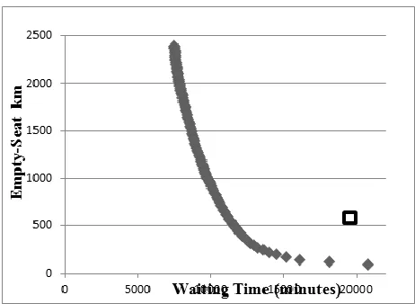
The results are shown in Figure 7. The final network contains about 100 dominant timetables, which are depicted in the Pareto frontier fashion. A single square data point (in black square around Empty-seat km=600 and Wait-time=20000 minutes) represents the current timetable. It can be seen that, using the proposed methodology, the waiting time for passengers can be improved by more than 43% for the same level of empty-seat km. It is worth noting that with the original timetable quite a few vehicles are overcrowded compared with the proposed procedure resulting without any overcrowding situations.

[image:7.612.329.560.471.640.2]

(8)

International Journal of Emerging Technology and Advanced Engineering

689

V. VEHICLE SCHEDULING WITH MULTI-VEHICLE TYPES

In the vehicle scheduling activity in Figure 1 the scheduler’s task is to list all daily chains of trips (some deadheading) for each vehicle so as to ensure the fulfillment of both timetable and operator requirements (refueling, maintenance, etc.). The major objective of this activity is to minimize the number of vehicles required in case of a single type, and minimum cost – for multi-type vehicles. The technique used is a step function termed deficit function, as it represents the deficit number of vehicles required at a particular terminal in a multi-terminal transit system [1,25]. The value of embarking on such a technique is to achieve the greatest saving in the number of vehicles and at the same time complying with passenger demand. This saving is attained through a procedure incorporating a man/computer interface allowing the inclusion of practical considerations that experienced transit schedulers may wish to introduce into the schedule.

A. Background on the Deficit Function

Following is a description of a step function approach described first by Ceder and Stern [25] and Ceder [1], for assigning the minimum number of vehicles to allocate for a given timetable. The step function is termed deficit function (DF), as it represents the deficit number of vehicles required at a particular terminal in a multi-terminal transit system. That is, DF is a step function that increases by one at the time of each trip departure and decreases by one at the time of each trip arrival. To construct a set of deficit functions, the only information needed is a timetable of required trips. The main advantage of the DF is its visual nature. Let

d k t S



, ,



denote the DF for the terminal

k

at the time

t

for the schedule

S

. The value of

d k t S



, ,



represents the total number of departures minus the total number of trip arrivals at terminal

k

, up to and including time

t

. The maximal value of

d k t S



, ,



over the schedule horizon



T T

₁

,

₂



is designated

D k S

 

,

.

Let

t

_si and

t

e i

denote the start and end times of trip

i

,

i



S

. It is possible to partition the schedule horizon of





d k t S

, ,

into sequence of alternating hollow and maximal intervals. The maximal intervals



s

_ik

,

e

_ik



,

i



1 ,...,

n

 

k

define the interval of time over which

d k t

 

,

takes on its maximum value.

Note that the

S

will be deleted when it is clear which underlying schedule is being considered. Index

i

represents the ith maximal intervals from the left and

n k

 

represents the total number of maximal intervals in

d k t

 

,

. A hollow interval

H

_lk, l=0 1 2 … n(k) is defined as the interval between two maximal intervals including the first hollow from T1 to the first maximal interval, and the last hollow-from the last interval to T2 . Hollows may consist of only one point, and if this case is not on the schedule horizon boundaries



T

₁ or

T

₂



, the graphical representation of

d k t

 

,

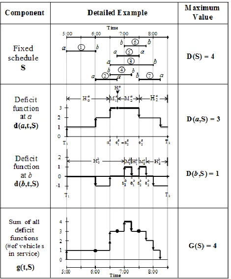
is emphasized by clear dot. Figure 8 illustrates these definitions.

If the set of all terminals is denoted as R, the sum of

 

D k

for all

k



R

is equal to the minimum number of vehicles required to service the set R. This is known as the fleet size formula. Mathematically, for a given fixed schedule S:

 

_ _

 

1,2

max

,

t T T

k R k R

D S

D k

d k t



 









(6)

Where

D S

 

is the minimum number of vehicles to service the set R.

When deadheading (DH) trips are allowed, the fleet size may be reduced below the level described in Equation (6). Ceder and Stern [25] described a procedure based on the construction of a unit reduction DH chain (URDHC), which, when inserted into the schedule, allows a unit reduction in the fleet size. The procedure continues inserting URDHCs until no more can be included or a lower boundary on the minimum fleet is reached. The lower boundary G(S) is determined from the overall deficit function defined as

 

_









T k

S

t

k

d

S

t

g

,

where

 

g

 

t

S

G

T T

t

max

,

)

(

2 1,





.

This function represents the number of trips simultaneously in operation. Initially, the lower bound was determined to be the maximum number of trips in a given timetable that are in simultaneous operation over the schedule horizon. Stern and Ceder [26] improved this lower bound, to

 

S

G

 

S

(9)

International Journal of Emerging Technology and Advanced Engineering

[image:9.612.53.288.201.485.2]

690 This lower bound was even further improved by Ceder [27] by looking into artificial extensions of certain trip-arrival points without violating the generalization of requiring all possible combinations for maintaining the fleet size at its lower bound.

Figure 8. Deficit functions of two-terminal fixed schedule

In addition, it is worth mentioning the NT (Next Terminal) selection rule and the URDHC routines. The selection of the next terminal in attempting to reduce its maximal deficit function may rely on the basis of garage capacity violation, or otherwise on a terminal whose first hollow is the longest. The rationale here is to try to open up the greatest opportunity for the insertion of the DH trip. Once a terminal k is selected, the algorithm searches to reduce D(k) using the URDHC routines. Then all the d(k,t)

are updated and the NT rule is again applied. In the URDHC routines there are four rules: (i) for inserting the DH trip manually in a conversational mode; (ii) for inserting the candidate DH trip which has the minimum travel time; (iii) for inserting a candidate DH trip whose hollow starts farthest to the right; and (iv) for inserting a candidate DH trip whose hollow ends farthest to the right.

In the automatic modes (ii), (iii), or (iv), if a DH trip cannot be inserted and the completion of a URDHC is blocked, the algorithm backs up to a DH candidate list and selects the next DH candidate on that list.

B. Optimization Framework of Vehicle-Type Scheduling Problem [30]

The problem, entitled the vehicle-type scheduling problem (VTSP), is based on given set S of trips (schedule) and set M of vehicle types, size- or type-based. The set M is arranged in decreasing order of vehicle cost so that if

M

u



is listed above

v



M

, it means that cu > cv, where cu, cv are the costs involved in employing vehicle types u and v, respectively. Each trip

i



S

can be carried out by vehicle type

u



M

or by other types listed prior to u in M.

The problem can be formulized as a cost-flow network problem, in which each trip is a node and an arc connects two trips if, and only if, it is possible to link them in a time sequence with and without DH connections. On each arc (i,j), there is a capacity of one unit and an assigned cost Cij. If the cost of the lower-level vehicle type associated with trip i is higher than the cost of the vehicle type (even if of a lower level) required for trip j, then Cij = ci. That is, Cij = max (ci,cj). The use of such a formulation was implemented by Costa et al. [28], who employed three categories of solutions: (a) a multi-commodity network flow; (b) a single-depot vehicle- scheduling problem; and (c) a set-partitioning problem with side constraints. The mixed-integer programming of these problems is known to be NP-complete as may be seen, for example, in Bertossi et al. [29]. The math-formulation concepts for the third category are further explained by Ceder [30].

(10)

International Journal of Emerging Technology and Advanced Engineering

691 The algorithm VTSP developed is heuristic in nature while incorporating all DF components. It is detailed in Ceder (2011). Because of the graphical features associated with DF theory, the algorithm can be applied in an interactive manner or in an automatic mode, along with the possibility of examining its intermediate steps. The following is an example used as an explanatory device for the description of algorithm VTSP.

The example is illustrated in Figure 9, and consists of 8 trips, three terminals (a,b,c), and three types of vehicles, with the cost of 12, 5, and3 cost-units, respectively. Figure 9(a) illustrates the simple network of routes, in which the DH travel time between each two terminals is 20 minutes. The timetable and trip travel times are shown in Figure 9(b) according to vehicle type. The DFs of algorithm VTSP for the example are depicted in Figure 9(c); all trips are served initially by the same vehicle type (Type 1). For inserting a DH trip, the NT rule (the first hollow is the longest) is applied; this results in the selection of terminal b. The URDHC procedure with Rule (ii) (furthest start of a hollow) then results in three DH trips, in which DH2 is used for the type. The DFs of algorithm VTSP for the example are depicted in Figure 9(c); all trips are served initially by the same vehicle type (Type 1). For inserting a DH trip, the NT rule (the first hollow is the longest) is applied; this results in the selection of terminal b. The URDHC procedure with Rule (ii) (furthest start of a hollow) then results in three DH trips, in which DH2 is used for the level of D(a). Two vehicle chains are then created using the FIFO [1-3-DH1-5-7] and [2-4-DH2-6-DH3-8], and the total cost is C1=24.

Algorithm VTSP continues with treating vehicle types separately. The maximum DF of Types 1 and 2 are reduced by one, using DH1 and DH2, respectively; the number of Type 3 vehicles remains same. Thus, N2 = 1 + 1 + 2 = 4, and the four following chains are derived by using the FIFO rule: [1-DH1-4] (vehicle type 1), [2-5-DH2-8] (vehicle type 2), [3-7], and [6] (vehicles of Type 3); this results in a total cost of C2 = 23.

[image:10.612.314.560.152.414.2]

The next step in algorithm VTSP compares N1 = 2 with N2 = 4, and then moves to the next step. Figure 10 (marked as part ‘e’ of the process) illustrates the process of this step which again applies the NT rule and the URDHC procedure with Rule (ii), but this time with the possibility of inserting any DH trip from a DF with a more expensive vehicle type to a DF with a less expensive type. The first terminal selected is b, based on d2(b,t), from which DH1 is determinedfrom terminal a.

[image:10.612.329.562.433.667.2]

Figure 9. Network, schedule and DFs of the example [30]

Figure 10. Min-cost solution [30] Time

Type 2 (c2=5)

Type 3 (c3=3) Type 1 (c1=12)

(b)

(a)

6:00 6:20 6:40 7:00 7:20 7:40 8:00 8:20 8:40 9:00 9:20 9:40

Time

d (c,t) d (b,t)

(c)

DH1

D(c) = 0 0

-1 -2 -3

d (a,t) D(a) = 1

DH2 DH₃

D(b) = 3 2 1

6:00 6:20 6:40 7:00 7:20 7:40 8:00 8:20 8:40 9:00 9:20 9:40

b b

a

b

a

b c

c c

a

a c

a b

c a

7 b

c a

8

6 5 3

4 2

1

(11)

International Journal of Emerging Technology and Advanced Engineering

692 The DFs are then updated and the next terminal again b,

but related to d1(b,t); DH2 is inserted from terminal c. It continues with the next selected terminal c, based on d3(c,t); however, no DH trip can be inserted into its maximum-interval starting point, including. Thus, a is selected next, based on d3(a,t), and DH3 is inserted to arrive from c, based on the updated d1(c,t). This terminates this step and results in the three following (FIFO) chains: [ 1-DH2-4-DH3-6] (vehicle type 1), [2-5-DH1-8] (vehicle Type 2), and [3-7] (vehicle Type 3), with a total cost of 12 + 5 + 3 = 20.

VI. CONCLUDING REMARK

This work, based on a keynote lecture given at the 14th EWGT (see Acknowledgement) is a mixture between reviewed and new methodologies including some case studies. It addresses a review of two transit operations-planning activities: timetable development and vehicle-scheduling with different vehicle sizes and types. Alternative timetables are constructed with either even headways, but not necessarily even passenger loads or even average passenger loads, but not even headways. A method to construct timetables with the combination of both even-headway and even-load is developed for multi-size vehicles. The vehicle-scheduling problem, called VSTP, is based on given sets of trips and vehicle types arranged in decreasing order of vehicle cost using the deficit-function theory. It is believed that prudent use of transit vehicles with different sizes cannot only make the service more reliable and attractive, but also can be more economical and save resources.

Acknowledgement

The author is grateful to Professor Jacek Zak and the organizers of the 14th EWGT and 26th Mini-EURO Conference at Poznan, Poland, 6-9 September, 2011, for their support of this article; it is based on the author’s keynote presentation at that conference.

REFERENCES

[1] Ceder, A. 2007. Public Transit Planning and Operation: Theory,

Modeling and Practice . Oxford, UK: Elsevier, Butterworth-Heinemann.

[2] Newell, G. F. 1971. Dispatching policies for a transportation route. Transportation Science, 5, 91-105.

[3] De Palma, A. and Lindsey, R. 2001. Optimal timetables for public transportation. Transportation Research, 35B, 789-813.

[4] Wirasinghe, S. C. 2003. Initial planning for an urban transit system.

In Advanced Modeling for Transit Operations and Service Planning (W. Lam and M. Bell, eds.), pp. 1-29, Pergamon Imprint, Elsevier Science Ltd. path problems.

[5] Adamski, A. 1998. Simulation support tool for real-time dispatching

control in public transport. Transportation Research, 32A (2), 73-87.

[6] Dessouky, M., Hall, R., Nowroozi, A., and Mourikas, K. 1999. Bus

dispatching at timed transfer transit stations using bus tracking technology. Transportation Research, 7C (4), 187-208.

[7] Furth, P.G. and Wilson, N.H.M. 1981. Setting frequencies on bus

routes: theory and practice. Transportation Research Record, 818, 1-7.

[8] Gallo, G. and Di-Miele, F. 2001. Dispatching buses in parking

depots. Transportation Science 35(3), 322-330.

[9] Ceder, A. 1986. Methods for creating bus timetables. Transportation

Research, 21A (1), 59-83.

[10] Löbel, A. 1999. Solving large-scale multiple-depot vehicle

scheduling problems. In Computer-Aided Transit Scheduling. Lecture Notes in Economics and Mathematical Systems, 471 (N. H. M. Wilson, ed.), pp. 193-220, Springer-Verlag.

[11] Freling, R., Wagelmans, A. P. M., and Paixao, J. M. P. 2001. Models

and algorithms for single-depot vehicle scheduling, Transportation Science, 35 (2), 165-180.

[12] Huisman, D., Freling, R., and Wagelmans, A.P.M. 2004. A robust

solution approach to the dynamic vehicle scheduling problem. Transportation Science, 38 (4), 447-458.

[13] Zak, J. A. 2009. Multiple criteria optimization method for the

vehicle assignment problem in a bus transportation company. Journal of Advanced Transportation .43(2) , 203-243.

[14] Borndorfer, R., Lobel, A., and Weider, S. 2008. A Bundle Method for Integrated Multi-Depot Vehicle and Duty Scheduling in Public Transit. In Computer-Aided Systems in Public Transport (M. Hickman, P. Mirchandani, S. Voss, eds). Lecture notes in economics and mathematical systems, Vol. 600, Springer, 3-24.

[15] Gintner, V., Kliewer, N. and Suhl, L. 2008. A Crew Scheduling

Approach for Public Transit Enhanced with Aspects from Vehicle Scheduling. In Computer-Aided Systems in Public Transport (M. Hickman, P. Mirchandani, S. Voss, eds). Lecture notes in economics and mathematical systems, Vol. 600, Springer, 25-42.

[16] Mesquita, M., Paias, A., and Respicio, A. 2009. Branching

Approaches for Integrated Vehicle and Crew Scheduling. Public Transport Planning and Operations 1(1), 21-37.

[17] Kwan R.S.K and Kwan A.S.K. 2007. Effective Search Space

Control for Large and/or Complex Driver Scheduling Problems. Annals of Operations Research 155, 417-435.

[18] Laplagne, I., Kwan R.S.K., and Kwan A.S.K. 2009. Critical Time

Window Train Driver Relief Opportunities. Public Transport planning and Operations 1(1), 73-85.

[19] Spicher, U. 2004. Skript zur Vorlesung Verbrennungsmotoren.

Karlsruhe,. Karlsruhe, Universitaet Karlsruhe, Institut für

Kolbenmaschinen. path problems.

[20] Potter, S. 2003. Transport energy and emissions: urban public

transport. Handbook of transport and the environment. D. A. Hensher and K. J. Button, Elsevier. 4, 247-263.

[21] Ceder, A., Hassold, S. and Dano, B. 2013. Approaching Even-Load

and Even-Headway Transit Timetables Using Different Bus Sizes. Journal of Public Transport – Planning and Operation; 5(3), 193-217.

[22] Hassold, S. and Ceder, A. 2012. Multiobjective Approach to

(12)

International Journal of Emerging Technology and Advanced Engineering

693

[23] Raith, A. and Ehrgott, M. 2009. A comparison of solution strategies

for biobjective shortest path problems. Computers & Operations Research, 36(4), 1299-1331.

[24] Brumbaugh-Smith, J. and Shier, D. 1989. An empirical investigation

of some bicriterion shortest path algorithms. European Journal of Operational Research. 43(2), 216-224.

[25] Ceder, A. and Stern, H.I. 1981. Deficit function bus scheduling with

deadheading trip insertion for fleet size reduction. Transportation Science, 15 (4), 338-363.

[26] Stern, H.I. & Ceder, A. 1983. An Improved Lower Bound to the Minimum Fleet Size Problem. Transportation Science, 17(4), 471-477.

[27] Ceder, A. 2002. A step function for improving transit operations planning using fixed and variable scheduling. In Transportation and Traffic Theory, (M.A.P. Taylor, ed), 1-21, Elsevier Science.

[28] Costa, A., Branco, I., and Paixao, J. 1995. Vehicle scheduling

problem with multiple types of vehicles and a single depot. In Computer-aided Transit Scheduling. Lecture Notes in Economics and Mathematical Systems, 430 (J. R. Daduna, I. Branco, and J. M. P. Paixao, eds.), pp. 115-129, Springer-Verlag.

[29] Bertossi, A., Carraresi, P., and Gallo, G. 1987. On some matching problems arising in vehicle scheduling. Networks, 17, 271-281.

[30] Ceder, A. 2011. Public-Transport Vehicle Scheduling with Multi