s a t ellit e c o n s t ell a ti o n d a t a fo r
m o ni t o ri n g w o o dl a n d i n t h e UK
O g u n b a d e w a , EY, Ar mi t a g e , R P a n d D a n s o n , F M
h t t p :// dx. d oi.o r g / 1 0 . 3 3 9 0 /f 5 0 7 1 7 9 8
T i t l e O p ti c al m e d i u m s p a ti al r e s ol u tio n s a t ellit e c o n s t ell a ti o n d a t a fo r m o n i t o ri n g w o o dl a n d i n t h e UK
A u t h o r s O g u n b a d e w a , EY, Ar mi t a g e , R P a n d D a n s o n , F M
Typ e Ar ticl e
U RL T hi s v e r si o n is a v ail a bl e a t :
h t t p :// u sir. s alfo r d . a c . u k /i d/ e p ri n t/ 3 2 1 0 6 / P u b l i s h e d D a t e 2 0 1 4
U S IR is a d i gi t al c oll e c ti o n of t h e r e s e a r c h o u t p u t of t h e U n iv e r si ty of S alfo r d . W h e r e c o p y ri g h t p e r m i t s , f ull t e x t m a t e r i al h el d i n t h e r e p o si t o r y is m a d e f r e ely a v ail a bl e o nli n e a n d c a n b e r e a d , d o w nl o a d e d a n d c o pi e d fo r n o
n-c o m m e r n-ci al p r iv a t e s t u d y o r r e s e a r n-c h p u r p o s e s . Pl e a s e n-c h e n-c k t h e m a n u s n-c ri p t fo r a n y f u r t h e r c o p y ri g h t r e s t r i c ti o n s .
forests
ISSN 1999-4907
www.mdpi.com/journal/forests
Article
Optical Medium Spatial Resolution Satellite Constellation Data
for Monitoring Woodland in the UK
Ebenezer Y. Ogunbadewa 1, Richard P. Armitage 2,* and F. Mark Danson 2
1 Geography Department, Adekunle Ajasin University Akungba-Akoko, 23401 Ondo-State, Nigeria; E-Mail: ogunbadewa202@yahoo.com
2 School of Environment and Life Sciences, University of Salford, Salford M5 4WT, UK; E-Mail: f.m.danson@salford.ac.uk
* Author to whom correspondence should be addressed; E-Mail: r.p.armitage@salford.ac.uk; Tel.: 44-161-295-5646.
Received: 7 March 2014; in revised form: 23 June 2014 / Accepted: 2 July 2014 / Published: 23 July 2014
Abstract: The aim of this study was to test the potential of a constellation of remote sensing satellites, the Disaster Monitoring Constellation (DMC), for retrieving a temporal record of forest leaf area index (LAI) in the United Kingdom (U.K.). Ground-based LAI measurements were made over a 12-month period in broadleaf woodland at Risley Moss Nature Reserve, Lancashire, U.K. The ground-based LAI varied between zero in January to a maximum of 4.5 in July. Nine DMC images, combining data from UK-DMC and NigeriaSat-1, were acquired, and all images were cross-calibrated and atmospherically corrected. The spectral reflectance of the test site was extracted, and a range of vegetation indices were then computed and correlated with the ground measurements of LAI. The soil adjusted vegetation index (SAVI) had the strongest correlation, and this was used to derive independent estimates of LAI using the “leave-one-out” method. The root mean square error of the LAI estimates was 0.47, which was close to that calculated for the ground-measured LAI. This study shows, for the first time, that data from a constellation of high temporal, medium spatial resolution optical satellite sensors may be used to map seasonal variation in woodland canopy leaf area index (LAI) in cloud-prone areas, like the U.K.
1. Introduction
Vegetation phenology is the temporal pattern of seasonal vegetation development, particularly leaves, and its subsequent senescence, as determined by variations in climate, day length and characteristics of the vegetation, such as species, and the environment, such as substrate [1–3]. Monitoring vegetation phenology over time is essential in understanding ecosystem, biological, biophysical, biogeochemical and energy processes and fluxes. Vegetation responds in cyclical ways to these processes, and therefore, variations in vegetation phenology can be linked to environmental change across a wide range of spatial and temporal scales [3–6]. Vegetation phenology is acknowledged as an essential source of information for understanding the impacts of climate change, due to the relationship between seasonal phenological changes and climatic factors, such as temperature, rainfall and snowfall [7–9]. However, in order to make use of vegetation phenology in examining the possible impacts of changes in the Earth’s climate, phenological measurements are required at a range of spatial scales, namely local, regional and global. Even though there are existing phenological records derived from traditional methods of in situ observations and process-based models, these phenological statistics have limited spatial coverage, due to very sparse networks, lack adequate baselines and uniformity in terminology and methodology, and present limited opportunities for the inter-comparison of observations across regions [2,10–16]. Therefore, there is a need for alternative methods to monitor vegetation phenology that will facilitate synoptic observations [17]. One approach that achieves this is the coupling of ground-based measurements of leaf area index (LAI) with spectral reflectance information, often expressed as vegetation indices (VI), derived from multi- and high-temporal satellite remote sensing imagery [6,18].
The leaf component of a vegetation canopy is a biophysical property that can be measured using the structural attribute, leaf area index (LAI) [19]. Variation in canopy LAI (leaf area per unit ground area) over time is related to the rate of expansion of leaf material, and as such, it is a good indicator of canopy phenology [5,19–22]. There are a number of direct and indirect methods to measure LAI. Direct measurement methods include full or partial harvesting of stands, the application of allometric equations and the use of leaf litter-fall collection. Indirect measurement methods include the use of instruments that estimate light transmittance through the canopy as a measure of LAI [23,24]. However, the limitations of all of these methods are that they only sample discrete locations or, at the very best, small areas, and they are usually limited in terms of temporal repeatability [25]. Remote sensing offers a potential approach to address these limitations, by providing spatial coverage and the repeatability of observation [26]. Relationships between LAI measurements on the ground and remote sensing estimates of vegetation phenology have been widely established [3,26–28].
(2005), there was an average probability of cloud-free viewing only 21.3% of the time, with a minimum probability of just 12.9% and a maximum of 33.3% of the time. This means that for a sensor like Landsat, which has a medium spatial resolution and a revisit period of 16 days, there would be approximately five cloud-free images a year, or fewer for some areas, of the U.K. The analysis [34] showed large spatial variations in cloud cover, with fewer cloud-free observing opportunities in the north and west of Great Britain in 2005 and more in the south. The potential limitations caused by cloud cover are problematic for applications requiring high observation frequencies, such as phenological measurements [35–39]. Therefore, ideally, satellite sensors with a high revisit frequency are required, but there is then likely to be a trade-off between this high temporal resolution and the spatial resolution of the sensor [40–42].
Satellite sensors with high temporal resolution tend to have coarse spatial resolution. These would include sensors, such as the Advanced Very High Resolution Radiometer (AVHRR), the Moderate Resolution Imaging Spectroradiometer (MODIS) and the Medium Resolution Imaging Spectrometer (MERIS), which have been used in numerous phenological studies [2,3,16–19,43–46]. These sensors have a daily revisit capability, but the spatial resolutions vary from 250 m to 1.1 km, which may be too coarse to capture the spatial variability in the vegetation cover. Medium spatial resolution sensors, which typically have a spatial resolution of the order of 20 to 30 m, have also been used for phenological studies [35,47,48]. These sensors have a suitable spatial resolution, but typically, their revisit period is measured in numbers of days, which leads to phenological events being missed. One approach that has been adopted for sensors with coarser temporal resolutions is to “fuse” data sets together from a number of different sensors [18], which has the effect of increasing the temporal resolution of the observations made. However, there are potential issues with the complexity of the inter-calibrations between any sensors used and also the time it is likely to take to generate a product, if the intention is to use the system for the operational monitoring of phenology. To date, there have been no phenological studies that have employed high temporal resolution data (daily repeat) from a medium spatial resolution sensor. The Disaster Monitoring Constellation (DMC) Satellite series, developed by Surrey Satellite Technology Ltd (SSTL), U.K., offers the opportunity to collect the types of time series data sets that are crucial in phenological studies at relatively high spatial resolution.
satellites were launched between 2002 and 2003 and have been followed by modified and upgraded systems. The potential that DMC offers for phenological studies is in the daily repeat cycle of image acquisition, coupled with a relatively high spatial resolution.
The research presented in this paper aims to investigate whether data from the Disaster Monitoring Constellation of satellites can be used to derive timely quantitative measures of vegetation dynamics at a local scale. The objectives are: (i) to determine whether vegetation indices derived from DMC data can be related to variations in LAI measured at ground level; and (ii) to determine whether these data provide accurate multi-temporal estimates of leaf area index (LAI) for a woodland site in the U.K.
2. Methods, Study Area and Data Analysis
The methods selected to address the objectives were to measure the seasonal variation in LAI in a broadleaved deciduous plot at a woodland site in north-west England and to use a series of DMC images to track the variations in LAI of the plot. Broadleaved deciduous woodland in the U.K. follows a clear phenological pattern with bud-burst in early spring, leaf development through to mid-summer, followed by senescence and eventual leaf fall in late autumn. This sequence thus exhibits a wide range of LAI states with which to test the applicability of the DMC data.
2.1. Study Site and Ground Data Collection
2.2. Satellite Image Data Analysis
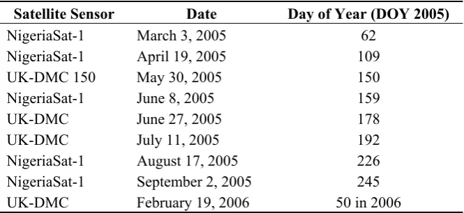
[image:6.595.132.465.293.446.2]DMC images of the study area were supplied as quick-looks by DMC International Imaging, and nine images were identified with a cloud-free view of the study site (Table 1). Four of the images were from the UK-DMC and five from NigeriaSat-1. The nine images represented a subset of the possible imaging opportunities. As with most commercial remote sensing sensors, the DMC Constellation collects data on a tasking basis, and so, not all targets are covered on every overpass of the satellites. In addition, the first generation of DMC satellite had limited on-board storage, and this coupled to a then limited network of ground receiving stations reduced the volume of data collected on each overpass. These factors meant that while it was theoretically possible to have daily images of the study area, the actual imagery available was more limited.
Table 1. List of the Disaster Monitoring Constellation (DMC) data sets.
Satellite Sensor Date Day of Year (DOY 2005)
NigeriaSat-1 March 3, 2005 62
NigeriaSat-1 April 19, 2005 109
UK-DMC 150 May 30, 2005 150
NigeriaSat-1 June 8, 2005 159
UK-DMC June 27, 2005 178
UK-DMC July 11, 2005 192
NigeriaSat-1 August 17, 2005 226
NigeriaSat-1 September 2, 2005 245
UK-DMC February 19, 2006 50 in 2006
The image for June 27, 2005, appeared on visual inspection to have both little cloud cover and the least haze. This image was thus selected as the base for the atmospheric correction procedure applied to all of the images. The June 27 image was geometrically corrected to the UTM WGS84 coordinate system by selecting 30 ground control points (GCPs) from U.K. Ordnance Survey maps. The image was resampled to a 32-m pixel size using nearest neighbour resampling Thereafter, this image was used to geometrically correct the other eight DMC images, using image to image geometric correction (Figure 1).
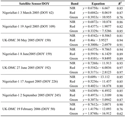
The June 27, 2005, image was atmospherically corrected using the COST (cosine of the solar zenith angle correction) model [55]. The COST model was applied to the image to convert it to estimated reflectance. The remaining eight DMC images were then cross-calibrated using this base image. Thirty homogeneous, flat, temporally- and spatially-stable objects, which were spectrally invariant, were used as targets in the calibration. The targets included dark objects, like black asphalt (major roads and airport runways) and water bodies, and brightly reflective objects, such as beaches. Antecedent surface conditions at each target were not explicitly accounted for, and so, some minor errors may have been introduced in to the corrections. The targets were used to derive regression equations of the cross-sensor reflectance calibration relationships [56,57] based on the equation:
where y is estimated reflectance, x is the digital number for the image and a and b are regression coefficients. Table 2 shows the regression equations for the individual images.
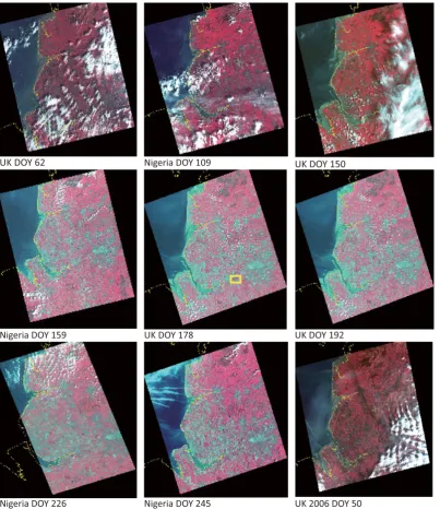
Figure 1. Geometrically-corrected DMC images used in this study; the images are displayed as false colour composites (red = DMC Band 1; green = DMC Band 2; blue = DMC Band 3); UK = UK-DMC, Nigeria = NigeriaSat-1; the yellow rectangle on DOY 178 shows the study area.
From each image, a single pixel was then identified corresponding to the centre of the Risley Moss sample plot and the green, red and near-infrared reflectance values extracted. The data analysis examined the linear regression relationships between the LAI of the test stand and a range of vegetation indices (VI) computed from the remotely sensed data. Results are reported here for three widely used VI, the normalised difference vegetation index (NDVI), the difference vegetation index (DVI) and the soil adjusted vegetation index (SAVI). After determining the strongest relationship, the
UK 2006 DOY 50 Nigeria DOY 245
Nigeria DOY 226
Nigeria DOY 159 UK DOY 178 UK DOY 192
UK DOY 150
Nigeria DOY 109
data were subjected to a leave-one-out cross-validation regression procedure [58] to determine independent estimates of LAI for each date. This method involved leaving out the data for one date and computing the regression relationship using all other dates; the process was repeated for all dates to give nine independent LAI estimates.
Table 2. Equations for image inter-calibration (n = 27).
Satellite Sensor/DOY Band Equation R2
NigeriaSat-1 3 March 2005 (DOY 62)
NIR y = 0.6758x − 6.667 0.85 Red y = 0.6042x− 8.0619 0.87 Green y = 0.3933x− 10.955 0.76
NigeriaSat-1 19 April 2005 (DOY 109)
NIR y = 0.6872x− 10.874 0.86 Red y = 0.4377x− 1.9077 0.82 Green y = 0.3329x− 7.5286 0.85
UK-DMC 30 May 2005 (DOY 150)
NIR y = 0.4542x + 0.5063 0.81 Red y = 0.46x− 3.9527 0.94 Green y = 0.3008x− 2.6979 0.91
NigeriaSat-1 8 June2005 (DOY 159)
NIR y = 0.6375x− 9.7863 0.94 Red y = 0.5919x− 6.1429 0.89 Green y = 0.4101x− 9.8495 0.89
UK-DMC 27 June 2005 (DOY 192)
NIR y = 0.7268x− 11.913 0.93 Red y = 0.5542x− 6.0036 0.97 Green y = 0.3171x− 2.8123 0.97
NigeriaSat-1 17 August 2005 (DOY 226)
NIR y = 0.609x− 13.112 0.85 Red y = 0.5236x − 11.437 0.85 Green y = 0.4021x− 16.878 0.80
NigeriaSat-1 2 September 2005 (DOY 245)
NIR y = 0.6349x− 6.4932 0.85 Red y = 0.4973x− 1.3109 0.96 Green y = 0.3073x− 5.0942 0.87
UK-DMC 19 February 2006 (DOY 50)
NIR y = 0.7612x− 3.0871 0.90 Red y = 1.4179x − 12.093 0.76 Green y = 1.8748x− 16.912 0.62
3. Results
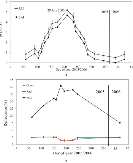
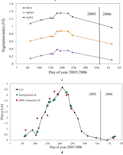
Figure 2. Temporal profiles of variation at the Risley Moss plot in (a) plant area index (PAI) and LAI (error bars are +/2 SD of PAI; (b) green, red and NIR reflectance; (c) three vegetation indices; (d) LAI and interpolated LAI at DMC collection dates (green circles) and estimated from DMC (red circles).
0 1 2 3 4 5 6
0 50 100 150 200 250 300 350 400 450
PA
I o
r
L
A
I
Day of year 2005/2006 PAI
LAI
2005 2006
85
29 July 2005
1 35
a
0 5 10 15 20 25 30 35 40 45
0 50 100 150 200 250 300 350 400 450
Refl
ect
an
ce (%
)
Day of year 2005/2006
Green
Red
NIR
35 85
1
2005
2006
Figure 2.Cont. 0 0.2 0.4 0.6 0.8 1 1.2 1.4 1.6
0 50 100 150 200 250 300 350 400 450
V
ege
ta
tion
inde
x (
V
I)
Day of year 2005/2006
DVI NDVI SAVI 35 85 1
2005
2006
c 0 0.5 1 1.5 2 2.5 3 3.5 4 4.5 50 50 100 150 200 250 300 350 400 450
PA I o r L A I
Day of year 2005/2006
LAI
Interpolated LAI
DMC estimated LAI
2005 2006
85
1 35
d
occurred around DOY 226 in 2005, with a reflectance of 39%, before it dropped back to about 18%. The general pattern was of increasing NIR during the growing season, with visible reflectance low over most of the growing cycle.
Figure 2c shows the temporal profile of the three vegetation indices derived from the DMC data for the study plot. The magnitude of the different indices varied, with NDVI having the highest values across the study period and DVI having the lowest. However, most important was that, even though they appeared noisy to some extent, the general form of the variation in the curves for the vegetation indices followed the trend in the LAI variation over the growing cycle. The minimum values for all three of the vegetation indices were found in February (DOY 50 in 2006), which coincided with an LAI value of around 0.2. The highest values for the three vegetation indices were in July, 2005 (DOY 192), which was very close to the highest value recorded for LAI, 4.67, measured at the study plot on DOY 210 in 2005. The range of variation in the three indices was very similar, with NDVI ranging from 0.51 to 0.96, SAVI ranging from 0.24 to 0.62 and DVI from 0.11 to 0.39. Correlation coefficients between LAI and the vegetation indices showed a significant positive relationship, with very little difference between the indices (Table 3). The implication that could be drawn from this is that the vegetation indices could be used to estimate LAI for the Risley Moss study plot.
Table 3. Linear correlation coefficients between measured LAI and vegetation indices (VI); all correlation coefficients were statistically significant (p < 0.01).
Vegetation Index r (n = 9)
Normalised difference vegetation index (NDVI) 0.92
Soil adjusted vegetation index (SAVI) Difference Vegetation Index (DVI)
0.94 0.93
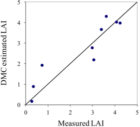
As SAVI had the strongest relationship with LAI, it was used in the leave-one-out cross-validation regression procedure to determine independent estimates of LAI for each date. The relationship between the LAI values estimated using the DMC-derived SAVI and the measured LAI values are shown in Figure 3. There was clearly a strong linear relationship between the predicted and the actual LAI values. For the study plot, Figure 3 indicates that there was some overestimation, where actual LAI is around one, and some underestimation for values around three. The over- and under-estimates generated a root mean square error of 0.47.
Figure 3. Relationship between measured LAI and LAI estimated from SAVI for the deciduous study plot at Risley Moss.
0 1 2 3 4 5
0 1 2 3 4 5
DM
C
e
stim
ate
d L
A
I
Measured LAI
4. Discussion
Previous research, such as White et al. [59], Jonsson and Eklundh [60], de Beurs and Henebry [61], Ganguly et al. [17] and Booker et al. [19], has demonstrated the potential of employing satellite remote sensing to monitor phenological events using vegetation indices linked to LAI. As was discussed earlier, two issues arise from the use of satellite data for phenological monitoring, namely the appropriateness of the spatial sampling (the spatial resolution) and whether imagery is available at the frequency required to measure phenological events. In studies, such as that carried out by Ganguly et al. [17] and Booker et al. [19], the remotely sensed data came from a sensor (MODIS) with a daily repeat cycle (high temporal resolution), but a coarse spatial resolution (pixels of the order of 250 m). Such sensors provide the frequency of observation required for phenological monitoring of U.K. forests, but the spatial resolution is not always appropriate, as noted by Booker et al. [19], Melaas et al. [62] and Tillack et al. [63]. Where the landscape is heterogeneous, such as typically found in natural and semi-natural woodland, results from coarse spatial resolution sensors have been shown to be less reliable in determining phenological events [64]. Melass et al. [62] demonstrated the potential of using finer spatial resolution imagery, from Landsat, to monitor phenology in woodland areas. In their study, Melass et al. [62] identified the start and the end of the growing season and were able to exploit a 30-year archive of Landsat imagery to demonstrate how these phenological events had varied over time.
covered by this study, there were only three cloud-free Landsat scenes available for the study area, making the monitoring of phenological changes impossible. The work presented in this paper indicates the potential of using a constellation of medium spatial resolution satellites that have the same or very similar imaging characteristics to Landsat. The advantage of the DMC constellation approach is that it combines the relatively high spatial characteristics (spatial resolution) required for looking at heterogeneous areas of vegetation, such as woodland, with the high frequency of observation (temporal resolution), due to the possibility of using the overpasses of multiple satellites, required for monitoring phenological events. While this research identified nine usable images, for the operational reasons noted earlier, it is estimated, using the work on cloud frequency of Armitage et al. [34], that with a daily overpass capability, the DMC satellites could have collected 76 cloud-free images over the study period if they had been tasked to do so.
The results obtained from the research presented here indicate a strong association between DMC-derived vegetation indices and LAI, the latter being a biophysical parameter that has already been shown to be suitable for monitoring phenology. The nature of the association between the DMC-derived vegetation indices and LAI is similar to that identified by Booker et al. [19],who found that LAI estimates produced from satellite imagery could be used to identify phenological changes in woodlands in southern England over a growing season. In a study looking at alluvial forests, Tillack et al. [63] found a strong relationship between vegetation indices derived from remote sensing and insitu LAI measured on the ground. Tillack et al. [63] noted that there was a non-linear temporal dimension to the relationship between vegetation indices and in situ LAI, and that during different phenological phases, different vegetation indices were more strongly correlated to LAI. This non-linear temporal relationship observed by Tillack. et al. [63] could explain the over- and under-estimations of LAI found in this study. Tillack et al. [63] noted the non-linear variation related to changing conditions in the canopy and environment (i.e., the visibility of the ground and understory; variations in shadow; changes in illumination conditions; etc.) and the impacts that these have on the calculation of the various vegetation indices. Further work is required in order to confirm whether the temporal variations in the LAI estimations observed in this research are due to similar factors, but it is likely that they are.
5. Conclusions
the potential to produce spectral indices that may be used to estimate LAI. Further work is required to look at how the temporal variations in LAI estimated from DMC relate to phenological events, and a greater frequency of images over the growing season would allow that.
Acknowledgments
DMC International Imaging Ltd. (DMCii) and the Nigerian National Space Research and Development Agency (NASRDA) are acknowledged for providing the DMC data; Gary Crowley (DMCii) kindly assisted in identifying suitable imagery and provided technical assistance. Risley Moss Local Nature Reserve is acknowledged for allowing access to the field site and providing logistical support for the field measurements.
Author Contributions
Ebenezer Y. Ogunbadewa conducted the fieldwork and image processing as part of his PhD research under the supervision of F. Mark Danson and Richard P. Armitage. For the initial draft of the paper Ebenezer Y. Ogunbadewa prepared the introduction and methods sections, Richard P. Armitage designed the results and discussion sections and F. Mark Danson produced the Figures. Richard P. Armitage was responsible for responding to the comments of the referees and co-ordinating the revisions to the paper.
Conflicts of Interest
The authors declare no conflict of interest.
References
1. Zhang, X.; Friedl, M.A.; Schaaf, C.B.; Strahler, A.H.; Hodges, J.C.F.; Gao, F.; Reed, B.C.; Huete, A. Monitoring vegetation phenology using MODIS. Remote Sens. Environ.2003, 84, 471–475. 2. Wolfe, D.W.; Schwartz, M.D.; Lakso, A.N.; Otsuki, Y.; Pool, R.M.; Shaulis, N.J. Climate change
and shifts in spring phenology of three horticultural woody perennials in northeastern USA.
Int. J. Biometeorol.2005, 49, 303–309.
3. Li, M.; Qu, J.J.; Hao, X. Investigating phenological changes using MODIS vegetation indices in deciduous broadleaf forest over continental U.S. during 2000–2008. Ecol. Inform. 2010, 5, 410–417.
4. Stockli, R.; Vidale, P.L. European plant phenology and climate as seen in a 20-year AVHRR land-surface parameter dataset. Int. J. Remote Sens.2004, 25, 3303–3330.
5. Arora, V.K.; Boer, G.J. A parameterization of leaf phenology for the terrestrial ecosystem component of climate models. Glob. Chang. Biol.2005, 11, 39–59.
6. Coops, N.C.; Hilker, T.; Bater, C.W.; Wulder, M.A.; Nielsen, S.E.; Mcdermid, G.; Stenhouse, G. Linking ground-based to satellite-derived phenological metrics in support of habitat assessment.
7. Walther, G.; Post, E.; Convey, P.; Menzel, A.; Parmesan, C.; Beedee, T.; Fromentin, J.; Hoegh-Guldberg, O.; Bairlein, F. Ecological responses to recent climate change. Nature 2002,
416, 389–395.
8. Parmesan, C.; Yohe, G. A globally coherent fingerprint of climate change impacts across natural systems. Nature2003, 421, 37–42.
9. Menzel, A.; Sparks, T.; Estrella, N.; Koch, E.; Aasa, A.; Ahas, R.; Alm-Kubler, K.; Bissolli, P.; Braslavska, O.; Briede, A. European phenological response to climate change matches the warming pattern. Glob. Chang. Biol.2005, 12, 1969–1976.
10. Sakai, R.K.; Fitzjarrald, D.R; Moore, K.E. Detecting leaf area and surface resistance during transition seasons. Agric. For. Meteorol.1997, 84, 273–284.
11. Sparks, T.; Jeffree, E.; Jeffree, C. An examination of the relationship between flowering times and temperature at the national scale using long-term phenological records from the UK.
Int. J. Biometeorol.2000, 44, 82–87.
12. Chmielewski, F.M.; Rötzer, T. Response of tree phenology to climate change across Europe.
Agric. For. Meteorol.2001, 108, 101–112.
13. Fitzjarrald, D.; Acevedo, O.; Moore, K. Climatic Consequences of Leaf Presence in the Eastern United States. J. Clim.2001, 14, 598–614.
14. Baldocchi, D.D. Assessing the eddy covariance technique for evaluating carbon dioxide exchange rates of ecosystems: Past, present and future. Glob. Chang. Biol.2003, 9, 479–492.
15. Jolly, W.M.; Nemani, R.; Running, S.W. A generalized, bioclimatic index to predict foliar phenology in response to climate. Glob. Chang. Biol.2005, 11, 619–632.
16. O’Connor, B.; Dwyer, E.; Cawkwell, F.; Eklundh, L. Spatio-temporal patterns in vegetation start of season across the island of Ireland using the MERIS Global Vegetation Index. ISPRS J. Photogramm. Remote Sens.2012, 68, 79–94.
17. Ganguly, S.; Friedl, M.A.; Tan, B.; Zhang, X.; Verma, M. Land surface phenology from MODIS: Characterization of the Collection 5 global land cover dynamics product. Remote Sens. Environ.
2010, 114, 1805–1816.
18. Verger, A.; Baret, F.; Weiss, M. A multisensor fusion approach to improve LAI time series.
Remote Sens. Environ.2011, 115, 2460–2470.
19. Booker, O.; Dash, J.; Dawson, T.P. Evaluation of leaf area index estimated from medium spatial resolution remote sensing data in a broadleaf deciduous forest in southern England, UK. Can. J. Remote Sens.2011, 37, 333–347.
20. Peña, M.A.; Brenning, A.; Sagredo, A. Constructing satellite-derived hyperspectral indices sensitive to canopy structure variables of a Cordilleran Cypress (Austrocedrus chilensis) forest.
ISPRS J. Photogramm. Remote Sens. 2012, 74, 1–10.
21. Chen, J.M.; Black, T.A. Defining leaf area index for non-flat leaves. Plant Cell Environ.1992, 15, 421–429.
23. Gower, S.; Kucharik, C.; Norman, J. Direct and indirect estimation of leaf area index, f (APAR), and net primary production of terrestrial ecosystems. Remote Sens. Environ.1999, 70, 29–51. 24. Breda, N.J.J. Ground-based measurements of leaf area index: A review of methods, instruments
and current controversies. J. Exp. Bot.2003, 54, 2403–2417.
25. Hufkens, K.; Friedl, M.; Sonnentag, O.; Braswell, B.H.; Milliman, T.; Richardson, A.D. Linking near-surface and satellite remote sensing measurements of deciduous broadleaf forest phenology.
Remote Sens. Environ.2012,117, 307–321.
26. Wang, Q.; Tenhunen, J.; Dinh, N.Q.; Reichstein, M.; Otieno, D.; Granier, A.; Pilegarrd K. Evaluation of seasonal variation of MODIS derived leaf area index at two European deciduous broadleaf forest sites. Remote Sens. Environ.2005, 96, 475–484.
27. Asner, G.P.; Scurlock, J.M.O.; Hicke, J.A. Global synthesis of leaf area index observations: Implications for ecological and remote sensing studies. Glob. Ecol. Biogeogr.2003, 12, 191–205. 28. Ahl, D.E.; Gower, S.T.; Burrows, S.N.; Shabanov, N.V.; Myneni, R.B.; Knyazikhin, Y. Monitoring
spring canopy phenology of a deciduous broadleaf forest using MODIS. Remote Sens. Environ.2006,
104, 88–95.
29. Cihlar, J.; Ly, H.; Li, Z.; Chen, J.; Pokrant, H.; Huang, F. Multitemporal, multichannel AVHRR data sets for land biosphere studies: Artifacts and corrections. Remote Sens. Environ. 1997, 60, 35–57.
30. Okin, G.S. Relative spectral mixture analysis—A multitemporal index of total vegetation cover.
Remote Sens. Environ.2007, 106, 467–479.
31. Song, C.; Schroeder, T.A.; Cohen, W.B. Predicting temperate conifer forest successional stage distributions with multitemporal Landsat Thematic Mapper imagery. Remote Sens. Environ.2007,
106, 228–237.
32. Busetto, L.; Meroni, M.; Colombo, R. Combining medium and coarse spatial resolution satellite data to improve the estimation of sub-pixel NDVI time series. Remote Sens. Environ.2008, 112, 118–131.
33. Kontoes, C.; Stakenborg, J. Availability of cloud-free Landsat images for operational projects. The analysis of cloud-cover figures over the countries of the European Community. Int. J. Remote Sens.
1990, 11, 1599–1608.
34. Armitage, R.P.; Ramirez, F.A.; Danson, F.M.; Ogunbadewa, E.Y. Probability of cloud-free observation conditions across Great Britain estimated using MODIS cloud mask. Remote Sens. Lett.
2013, 4, 427–435.
35. Fisher, J.I.; Mustard, J.F.; Vadeboncoeur, M.A. Green leaf phenology at Landsat resolution: Scaling from the field to the satellite. Remote Sens. Environ.2006, 100, 265–279.
36. Yang, W.; Shabanov, N.; Huang, D.; Wang, W.; Dickinson, R.; Nemani, R.; Knyazikhin, Y.; Myneni, R. Analysis of leaf area index products from combination of MODIS Terra and Aqua data. Remote Sens. Environ.2006, 104, 297–312.
37. Bontemps, S.; Bogaert, P.; Titeux, N.; Defourny, P. An object-based change detection method accounting for temporal dependences in time series with medium to coarse spatial resolution.
38. Huete, A.; Restrepo-Coupe, N.; Ratana, P.; Didan, K.; Saleska, S.; Ichii, K.; Panuthai, S.; Gamo, M. Multiple site tower flux and remote sensing comparisons of tropical forest dynamics in Monsoon Asia. Agric. For. Meteorol.2008, 148, 748–760.
39. Soundani, K.; le Maire, G.; Dufrêne, E.; François, C.; Delpierre, N.; Ulrich, E.; Cecchini, S. Evaluation of the onset of green-up in temperate deciduous broadleaf forests derived from Moderate Resolution Imaging Spectroradiometer (MODIS) data. Remote Sens. Environ. 2008,
112, 2643–2655.
40. Simoniello, T.; Carone, M.T.; Lanfredi, M.; Macchiato, M.; Cuomo, V. Landscape-scale characterization of vegetation phenology by using AVHRR-NDVI and Landsat-TM data.
Remote Sens. Agric. Ecosyst. Hydrol. V2004, 5232, 644–651.
41. Beck, P.S.A.; Atzberger, C.; Hogda, K.A.; Johansen, B.; Skidmore, A.K. Improved monitoring of vegetation dynamics at very high latitudes: A new method using MODIS NDVI. Remote Sens. Environ.2006, 100, 321–334.
42. Lunetta, R.S.; Knight, J.F.; Ediriwickrema, J.; Lyon, J.G.; Worthy, L.D. Land-cover change detection using multi-temporal MODIS NDVI data. Remote Sens. Environ.2006, 105, 142–154. 43. Duchemin, B. NOAA/AVHRR Bidirectional Reflectance: Modeling and Application for the
Monitoring of a Temperate Forest. Remote Sens. Environ.1999, 67, 51–67.
44. Hansen, M.C.; Townshend, J.R.G.; Defries, R.S.; Carroll, M. Estimation of tree cover using MODIS data at global, continental and regional/local scales. Int. J. Remote Sens. 2005, 26, 4359–4380.
45. Dash, J.; Mathur, A.; Foody, G.M.; Curran, P.J.; Chipman, J.W.; Lillesand, T.M. Land cover classification using multi-temporal MERIS vegetation indices. Int. J. Remote Sens. 2007, 28, 1137–1159.
46. Stow, D.; Petersen, A.; Hope, A.; Engstrom, R.; Coulter, L. Greenness trends of Arctic tundra vegetation in the 1990s: Comparison of two NDVI data sets from NOAA AVHRR systems.
Int. J. Remote Sens.2007, 28, 4807–4822.
47. Telesca, L.; Lasaponara, R. Quantifying intra-annual persistent behaviour in SPOT-VEGETATION NDVI data for Mediterranean ecosystems of southern Italy. Remote Sens. Environ. 2006, 101, 95–103.
48. Guyon, D.; Guillot, M.; Vitasse, Y.; Cardotd, H.; Hagolle, O.; Delzon, S.; Wigneron, J.-P. Monitoring elevation variations in leaf phenology of deciduous broadleaf forests from SPOT/VEGETATION time-series. Remote Sens. Environ.2011, 115, 615–627.
49. Sweeting, M.N.; Chen, F.Y. Network of Low Cost Small Satellites for Monitoring and Mitigation of Natural Disasters. In Proceedings of the 47th International Astronautical Congress, Beijing, China, 1996.
50. Stephens, J.P.; Sweeting, M. Developing a commercial interface for DMC data. In Proceedings of the 55th International Astronautical Congress, Vancouver, BC, Canada, 4–8 October 2004.
51. Da Silva Curiel, A.; Boland, L.; Cooksley, J.; Bekhti, M.; Stephens, P.; Sun, W.; Sweeting, M. First results from the disaster monitoring constellation (DMC). Acta Astronaut.2005, 56, 261–271.
53. Underwood, C.; Machin, S.; Stephens, P.; Hodgson, D.; da Silva Curiel, A.; Sweeting, M. Evaluation of the Utility of the Disaster Monitoring Constellation in Support of Earth Observation Applications. In the Proceedings of IAA Small Satellites for Earth Observation, Berlin, Germany, 2005; pp. 4–8.
54. Chen, J.; Cihlar, J. Plant canopy gap-size analysis theory for improving optical measurements of leaf-area index. Appl. Opt.1995, 34, 6211–6211.
55. Chavez, P.S. Image-based atmospheric corrections—Revisited and Improved. Photogramm. Eng. Remote Sens.1996, 62, 1025–1036.
56. Smith, G.; Milton, E. The use of the empirical line method to calibrate remotely sensed data to reflectance. Int. J. Remote Sens.1999, 20, 2653–2662.
57. Perry, E.; Warner, T.; Foote, P. Comparison of atmospheric modelling versus empirical line fitting for mosaicking HYDICE imagery. Int. J. Remote Sens.2000, 21, 799–803.
58. Geisser, S. The predictive sample reuses method with applications. J. Am. Stat. Assoc. 1975, 70, 329–328.
59. White, M.A.; Thornton, P.E.; Running, S.W. A continental phenology model for monitoring vegetation responses. Glob. Biogeochem. Cycles1997, 11, 217–234.
60. Jonsson, P.; Eklundh, L. Seasonality extraction by function fitting to time-series of satellite sensor data. IEEE Trans. Geosci. Remote Sens.2002, 40, 1824–1832.
61. De Beurs, K.M.; Henebry, G.M. Spatio-temporal statistical methods for modelling land surface phenology. In Phenological Research: Methods for Environmental and Climate Change Analysis; Hudson, I.L., Keatley, M.R., Eds.; Springer: Dordrecht/Heidelberg, Germany, 2010; pp. 177–208. 62. Melaas, E.K.; Friedl, M.A.; Zhu, Z. Detecting interannual variation in deciduous broadleaf forest
phenology using Landsat TM/ETM+ data. Remote Sens. Environ.2013, 132, 176–185.
63. Tillack, A.; Clasen, A.; Kleinschmit, B.; Förster, M. Estimation of the seasonal leaf area index in an alluvial forest using high-resolution satellite-based vegetation indices. Remote Sens. Environ.
2014, 141, 52–63.
64. Liang, L.; Schwartz, M.D.; Fei, S. Validating satellite phenology through intensive ground observation and landscape scaling in a mixed seasonal forest. Remote Sens. Environ. 2011, 115, 143–157.
65. Sandau, R. Status and trends of small satellite missions for earth observation. Acta Astronaut.
2010, 66, 1–12.