comm
en
t
re
v
ie
w
s
re
ports
de
p
o
si
te
d r
e
se
a
rch
refer
e
e
d
re
sear
ch
interacti
o
ns
inf
o
rmation
Ranked prediction of p53 targets using hidden variable dynamic
modeling
Martino Barenco
*†
, Daniela Tomescu
*
, Daniel Brewer
*†
, Robin Callard
*†
,
Jaroslav Stark
†‡
and Michael Hubank
*†
Addresses: *Institute of Child Health, University College London, Guilford Street, London WC1N 1EH, UK. †CoMPLEX (Centre for Mathematics
and Physics in the Life Sciences and Experimental Biology), University College London, Stephenson Way, London, NW1 2HE, UK. ‡Department
of Mathematics, Imperial College London, London SW7 2AZ, UK.
Correspondence: Michael Hubank. Email: m.hubank@ich.ucl.ac.uk
© 2006 Barenco et al.; licensee BioMed Central Ltd.
This is an open access article distributed under the terms of the Creative Commons Attribution License (http://creativecommons.org/licenses/by/2.0), which permits unrestricted use, distribution, and reproduction in any medium, provided the original work is properly cited.
p53 target prediction
<p>Hidden Variable Dynamic Modelling is a new approach to microarray analysis that quantitatively predicts the regulation of gene activ-ity.</p>
Abstract
Full exploitation of microarray data requires hidden information that cannot be extracted using current analysis methodologies. We present a new approach, hidden variable dynamic modeling (HVDM), which derives the hidden profile of a transcription factor from time series microarray data, and generates a ranked list of predicted targets. We applied HVDM to the p53 network, validating predictions experimentally using small interfering RNA. HVDM can be applied in many systems biology contexts to predict regulation of gene activity quantitatively.
Background
In order to understand how gene networks function, it is nec-essary to identify their components and to quantitatively describe how they relate to one another [1-3]. Subsequent prediction of gene network behavior requires identification of important parameters and variables, and estimation or meas-urement of their values during a response [4-6].
Experimental approaches can be applied to identify network components. For example, protein binding arrays and chro-mosome immunoprecipitation can be applied to identify transcription factor (TF)-binding sites and therefore infer TF targets [7-10]. However, these approaches give a static view of the system. Binding sites identified in vitro may not be avail-able in vivo, and different regulators may be active in differ-ent cellular systems. Furthermore, purely experimdiffer-ental approaches cannot predict in a quantitative manner, and with statistical confidence, the dynamics of network activity
with-out making an impractical number of experimental observa-tions [11].
Insight into the dynamic relationships present in a transcrip-tional response can be gained by running time series of microarrays [3,11,12]. Currently, analysis of this type of datum chiefly relies on clustering or correlation methods. The assumption is that groups of genes with similar expression profiles over time are likely to be regulated by the same TF. Although clustering approaches have been applied with some success, they are limited and inaccurate. Genes with different profiles may still be regulated by the same TF, and many genes included in clusters may be regulated by other factors. Clustering approaches typically do not generate confidence statistics about the validity of individual predictions, and therefore they can neither rank candidates nor distinguish between true and false targets.
Published: 31 March 2006
Genome Biology 2006, 7:R25 (doi:10.1186/gb-2006-7-3-r25)
Received: 24 November 2005 Revised: 30 January 2006 Accepted: 21 February 2006 The electronic version of this article is the complete one and can be
Importantly, because clustering is based on only the expres-sion time profile, the influence of other important factors required to reconstruct gene network activity is not taken into account. For example, transcript degradation rates, the sensi-tivity of a gene to a TF (or affinity of binding to the promoter), and the activity of the TF itself all contribute to the overall transcriptional output. Where clustering methods alone are applied, these quantities remain hidden in the data and are likely to confound any attempted analysis. As a consequence, microarray experiments typically return a list of targets based on expression level alone, and prioritization of genes of inter-est depends chiefly on researcher intuition.
An alternative strategy is to use a mathematical model of the network dynamics to provide a framework for the analysis of the expression time profile. Several types of model have been applied at different levels of complexity ranging from parts lists to dynamic models [3,11,12]. In theory, modeling can be applied to reconstruct a gene network in a quantitative man-ner [3,11,13]. The advantage of such an approach is that all of the important mechanisms that affect transcript levels can be taken into account simultaneously. Statistical confidence intervals can then be calculated, which allow the prediction of transcriptional targets with a specified statistical significance. As a result it is possible to predict how network regulation would change in response to differing conditions, allowing the optimal targeting of expensive experimental approaches.
We therefore developed a mathematical approach that uses information from a dynamic microarray time series data set to estimate, with confidence intervals, key parameters and hidden variables, specifically TF activity profiles. We define TF activity in terms of the positive effect that the TF has on transcription of its targets. We chose as a model experimental system the transcriptional response to ionizing irradiation. Ionizing radiation induces DNA damage, which in turn acti-vates the p53 response [14]. p53 is a transcription factor and tumor suppressor, but it is only one of several TFs activated by DNA damage [15,16].
Our analysis method allows quantitative prediction, with con-fidence, of transcripts that are upregulated by p53 in the com-plex response, without the need for very large numbers of experimental observations. We have made use of prior bio-logic information (known p53 targets) to construct a mathe-matical model of gene regulation, calculated confidence intervals using a highly efficient novel approach, and anchored the model by including a surprisingly small amount of additional biologic information. We show that the model outperforms a clustering approach in terms of accuracy of tar-get prediction, and we successfully tested model predictions with a separate experimental data set.
Results
A model of transcription factor-dependent gene transcription
We grew and irradiated a human leukemia cell line (MOLT4) containing functional p53 and harvested protein and RNA at regular intervals after irradiation. The time course was
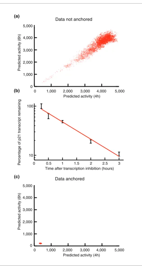
[image:2.612.317.556.82.531.2]per-Model based estimation of activity profile of p53 Figure 1
Model based estimation of activity profile of p53. (a) Markov Chain Monte Carlo output for potential transcription factor activity profile values for first time series replicate at 4 hours (x axis) and 6 hours (y axis). (b) Concentration of p21WAF1 transcript determined by real-time polymerase
chain reaction after addition of actinomycin D (10 µg/ml) to irradiated (5 Gy, 4 hours) MOLT4 cells cultured in RPMI. Expressed as percentage of initial concentration. (c) Using the degradation rate of p21WAF1
dramatically restricted the range of solutions to the Markov Chain Monte Carlo.
Data not anchored
5,000
2,000 1,000 1,000
2,000 3,000 4,000
5,000 4,000 3,000
1 0.5 10 100
Predicted activity (4h)
Predicted activity (6h)
3 2.5 2 1.5
P
e
rcentage of p21 tr
anscr
ipt remaining
Time after transcription inhibition (hours) 0
0 0
Data anchored
5,000
2,000 1,000 1,000
2,000 3,000 4,000
5,000 4,000 3,000 Predicted activity (4h)
Predicted activity (6h)
0 0
(a)
comm
en
t
re
v
ie
w
s
re
ports
refer
e
e
d
re
sear
ch
de
p
o
si
te
d r
e
se
a
rch
interacti
o
ns
inf
o
rmation
formed in triplicate, and Affymetrix U133A microarrays (Affymetrix Inc., Santa Clara, CA, USA) were run to measure the global transcriptional response. Before irradiation, we assumed the p53 network to be in equilibrium (that is, that the rate of change in its constituents is zero). Irradiating the cells disrupts the equilibrium and activates transcription of numerous p53 target genes. The rate at which p53-dependent mRNA transcripts accumulate depends on the basal tran-scription rate of a target gene, the sensitivity of the gene to p53, the level of activity of p53, and the transcript degradation rate. We can connect these factors to represent the overall behavior of the system. The time evolution of each gene tran-script is described by the following non-autonomous linear
differential equation for the rate of change in transcript con-centration xj(t) of gene j at time t:
Where Bj is the constant basal transcription rate of j; Sjf(t) is the transcription induced by p53, composed of a constant Sj, which is the sensitivity of gene j to p53, and f(t), which is the activity of p53 at time t; and Djxj(t) is a degradation term, with Dj being a constant degradation rate. For a full description of the model, see Mathematical methodology (below).
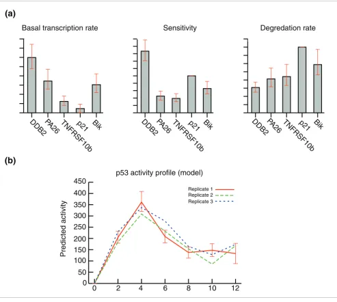
[image:3.612.61.554.86.528.2]Parameter estimation for a training set of five known p53 targets Figure 2
Parameter estimation for a training set of five known p53 targets. (a) The model equation was solved to estimate values for the parameters basal transcription Bj sensitivity Sj, and degradation Dj for the five p53 targets DDB2, p21WAF1/CIP1, SESN1/hPA26, BIK, and TNFRSF10b/TRAILreceptor 2. (b)
Simultaneously, the activity profile f(t) of p53 was derived from three separate microarray time courses.
50
6
4
2
0
0
400
350
300
250
200
150
100
Bik
p21
TNFRSF10b
PA
26
DDB2
p53 activity profile (model)
Predicted activity
450
12
10
8
Replicate 1
Replicate 3 Replicate 2
Bik
p21
TNFRSF10b
PA26
DDB2
DDB2
PA26
TNFRSF10b
p21
Bik
(a)
(b)
Degredation rate
Sensitivity
Basal transcription rate
dx t
dt B S f t D x t model equation
j
j j j j
( )
( ) ( )
Deriving the hidden activity profile of p53
In order to predict whether a gene is likely to be a p53 target, it is necessary to estimate its sensitivity (Sj) to p53 and to ensure that parameter values can be found that, when com-bined in the model equation, result in an expression profile similar to the experimentally determined profile. However, the p53 activity f(t) is not experimentally available and is the key 'hidden variable' in the system. To estimate this profile we used prior biologic knowledge rather than adopting a 'black box' approach. We selected a small training set of five known p53 targets (DDB2, p21WAF1/CIP1, SESN1/hPA26, BIK, and
TNFRSF10b/TRAILreceptor 2) [17-22] and used the
micro-array time series observations for this set to derive the p53 activity profile f(t), and the parameter values of basal tran-scription rate, sensitivity to p53, and degradation rate. These values and their confidence intervals were obtained by apply-ing Markov Chain Monte Carlo (MCMC) with a Metropolis-Gibbs sampler [23] (see Mathematical methodology, below). Normally, the calculations involved in these estimations are very demanding on computer time. In terms of systems biol-ogy, in which many such calculations are likely to be linked, this poses a major barrier to network analysis. We therefore discretized the model equation and devised a fast matrix-based algorithm to solve it efficiently (see Mathematical methodology, below).
Initial estimates of the parameters and the hidden profile f(t) exhibited a very high degree of variance. Repeated modeling of artificial data indicated that this was a general characteris-tic of the model and not peculiar to the parcharacteris-ticular experimen-tal data set. We noticed that the estimates were highly correlated with each other (Figure 1a). This suggested that experimentally determining the value of one additional parameter might constrain the others and so reduce the over-all variance. We therefore measured the rate of degradation of one transcript (p21WAF1/CIP1) using quantitative polymerase
chain reaction (PCR; Figure 1b). We found that this single measurement was sufficient to reduce dramatically the vari-ance and greatly improve the final estimates (Figure 1c). We term this process 'data anchoring'. We found that obtaining the degradation rate of any element in the training set was equally sufficient to anchor the model, provided that the same gene was also used as the reference point for estimating sen-sitivity (see Mathematical methodology, below). The
[image:4.612.314.559.85.425.2]inclu-Experimentally determined p53 activity profile Figure 3
Experimentally determined p53 activity profile. The activity profile of p53 was measured by Western blot to determine the levels of ser-15 phosphorylated p53 (ser15P-p53). ser-15 phosphorylation is a measure of p53 activity. IR, ionizing radiation. IR, ionizing irradiation.
Time (h) 4
2 0 0 0.2 0.4 0.6 0.8 1 1.2
12 10 8 6 4 2 0
Actin ser15P-p53
5 Gy IR (h)
12 10 8 6
Relative density
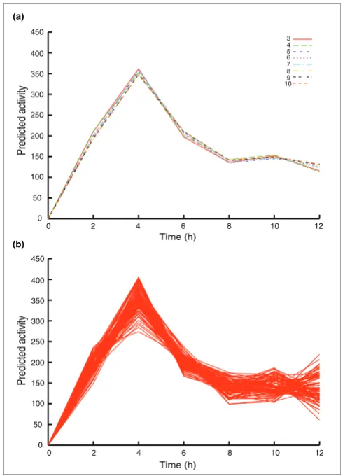
[image:4.612.57.302.87.351.2]Choice and number of training set genes does not significantly affect the predicted activity profile
Figure 4
Choice and number of training set genes does not significantly affect the predicted activity profile. (a) Predicted activity profile of p53 derived using different numbers of known targets in the training set, from three to ten genes. (b) Predicted activity profile of p53 derived using 100 combinations of three randomly selected training set genes from a pool of 10 known targets.
Time (h)
Time (h)
Predicted activity
Predicted activity
450
3
12 0
0
10 8 6 4 2 50
100 150 200 250 300 350 400
4 5
10 9 8 7 6 (a)
(b)
450
12 0
0
10 8 6 4 2 50
comm
en
t
re
v
ie
w
s
re
ports
refer
e
e
d
re
sear
ch
de
p
o
si
te
d r
e
se
a
rch
interacti
o
ns
inf
o
rmation
sion of the degradation rates of more genes did not significantly improve parameter estimation.
Incorporation of the degradation data allowed efficient esti-mation of the parameters Bj, Sj and Dj, and the p53 activity profile f(t) for the training set of known targets (Figure 2). This process was performed simultaneously on three repli-cate time series to improve the robustness of the outcome (Figure 2b). We found that the model-estimated profile approximated the experimentally determined activity profile
based on measuring p53 phosphorylation at serine 15 [24] (Figure 3). The profiles show a close match early in the response, but the model predicts a more rapid decline in activity. This discrepancy can be explained by the operation of other regulatory mechanisms that affect p53 activity but not concentration, for example relocation of phosphorylated p53 to the cytoplasm [25].
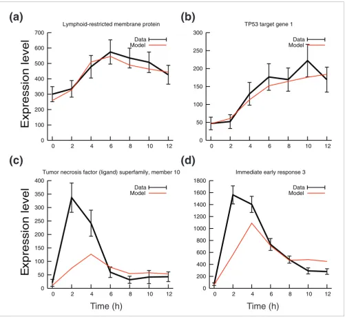
[image:5.612.55.556.85.545.2]Hidden variable dynamic modeling screening of upregulated genes Figure 5
Hidden variable dynamic modeling screening of upregulated genes. Model predicted profile (red) and experimental expression profile (black) of typical genes representing two classes of model prediction (class 1 and class 2). (a) Class 1 genes with good model score (M < 100) and high sensitivity P value (sensitivity Z score > 2; for example LRMP). (b) Class 1 genes with atypical expression profiles (for example, p53TG1); this profile occurs because of a low predicted degradation rate. (c,d) Two class 2 genes with low model score (M > 100) but high sensitivity P value (sensitivity Z score > 2; for example, TNFSF10 and IER3).
0 100 200 300 400 500 600 700
0 2 4 6 8 10 12
Lymphoid-restricted membrane protein
Data Model
0 50 100 150 200 250 300
0 2 4 6 8 10 12
TP53 target gene 1
Data Model
0 50 100 150 200 250 300 350 400
0 2 4 6 8 10 12
Tumor necrosis factor (ligand) superfamily, member 10
Data Model
0 200 400 600 800 1000 1200 1400 1600 1800
0 2 4 6 8 10 12
Immediate early response 3
Data Model
(b)
(a)
(d)
(c)
pression level
x
E
Expression level
)
h
(
e
m
i
T
)
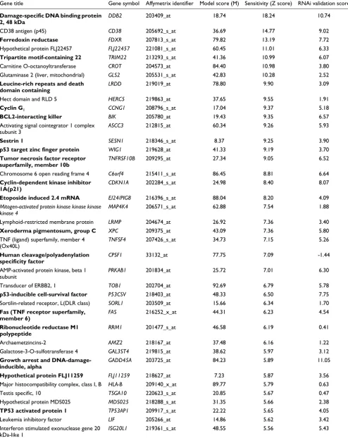
Table 1
Top 50 genes predicted by hidden variable dynamic modeling to be p53 regulated, ranked by sensitivity Z score
Gene title Gene symbol Affymetrix identifier Model score (M) Sensitivity (Z score) RNAi validation score
Damage-specific DNA binding protein 2, 48 kDa
DDB2 203409_at 18.74 18.24 10.74
CD38 antigen (p45) CD38 205692_s_at 36.69 14.77 9.02
Ferredoxin reductase FDXR 207813_s_at 79.82 13.19 7.72
Hypothetical protein FLJ22457 FLJ22457 221081_s_at 60.45 11.01 6.33
Tripartite motif-containing 22 TRIM22 213293_s_at 41.36 10.99 6.07
Carnitine O-octanoyltransferase CROT 204573_at 84.40 10.98 3.80
Glutaminase 2 (liver, mitochondrial) GLS2 205531_s_at 42.83 10.28 2.52
Leucine-rich repeats and death domain containing
LRDD 219019_at 78.80 9.90 3.09
Hect domain and RLD 5 HERC5 219863_at 37.65 9.55 1.91
Cyclin G1 CCNG1 208796_s_at 17.04 9.37 5.18
BCL2-interacting killer BIK 205780_at 19.43 9.35 6.57 Activating signal cointegrator 1 complex
subunit 3
ASCC3 212815_at 60.34 9.26 5.93
Sestrin 1 SESN1 218346_s_at 8.37 9.25 3.90
p53 target zinc finger protein WIG1 219628_at 41.33 9.19 3.70
Tumor necrosis factor receptor superfamily, member 10b
TNFRSF10B 209295_at 27.34 9.05 6.52
Chromosome 6 open reading frame 4 C6orf4 215411_s_at 86.45 8.81 6.64
Cyclin-dependent kinase inhibitor 1A(p21)
CDKN1A 202284_s_at 24.98 8.40 8.07
Etoposide induced 2.4 mRNA EI24/PIG8 216396_s_at 88.04 8.20 4.09
Mitogen-activated protein kinase kinase kinase kinase 4
MAP4K4 206571_s_at 62.88 7.54 1.88
Lymphoid-restricted membrane protein LRMP 204674_at 26.92 7.36 3.40
Xeroderma pigmentosum, group C XPC 209375_at 43.09 7.36 5.80 TNF (ligand) superfamily, member 4
(Ox40L)
TNFSF4 207426_s_at 34.73 7.15 5.26
Human cleavage/polyadenylation specificity factor
CPSF1 33132_at 77.75 7.09 -1.44
AMP-activated protein kinase, beta 1 subunit
PRKAB1 201834_at 25.72 7.01 6.30
Transducer of ERBB2, 1 TOB1 202704_at 92.69 6.79 5.78
p53-inducible cell-survival factor P53CSV 218403_at 48.33 6.50 7.75
Sortilin-related receptor, L(DLR class) SORL1 203509_at 15.66 6.34 1.70
Fas (TNF receptor superfamily, member 6)
FAS 216252_x_at 44.31 6.23 4.54
Ribonucleotide reductase M1 polypeptide
RRM1 201477_s_at 46.58 6.19 0.41
Archaemetzincins-2 AMZ2 218167_at 37.48 6.16 1.22
Galactose-3-O-sulfotransferase 4 GAL3ST4 219815_at 38.62 5.97 3.12
Growth arrest and DNA-damage-inducible, alpha
GADD45A 203725_at 84.23 5.89 11.05
Hypothetical protein FLJ11259 FLJ11259 218627_at 7.23 5.87 3.56
Major histocompatibility complex, class I, B HLA-B 209140_x_at 89.77 5.79 0.63
Testis specific, 10 TSGA10 220623_s_at 20.85 5.67 0.47
Hypothetical protein MDS025 MDS025 218288_s_at 31.35 5.66 2.38
TP53 activated protein 1 TP53AP1 209917_s_at 22.22 5.65 4.05
Leukemia inhibitory factor LIF 205266_at 14.86 5.62 3.42
Interferon stimulated exonuclease gene 20 kDa-like 1
comm
en
t
re
v
ie
w
s
re
ports
refer
e
e
d
re
sear
ch
de
p
o
si
te
d r
e
se
a
rch
interacti
o
ns
inf
o
rmation
Optimization of the model
The use of a training set of known targets takes advantage of the fact that prior biologic knowledge exists for many TFs. Because the p53 response is well studied, we were able to examine the optimum model requirements. We found that three training genes are sufficient for the model to make accu-rate parameter estimates (Figure 4a). The inclusion of more (up to ten) genes narrowed the confidence intervals but the improvement was small beyond five genes. We also found that inclusion of genes not regulated by p53 (for example
TNFSF10) led to a poor gene-specific model score, enabling
these genes to be excluded from the training set. We found the method to be very robust, and the exact choice of target genes does not appear to affect estimation greatly, providing that the measurement error is not excessive (namely, the detec-tion P value should be below 0.001 for Affymetrix data) and that the anchoring gene is clearly differentially regulated (Figure 4b; also see Mathematical methodology, below).
Prediction of p53 targets using hidden variable dynamic modeling
Once we had constructed the estimate for the key 'hidden var-iable', namely the p53 activity profile f(t), we were able to apply the model to the remaining expression data to predict p53 targets. Data was filtered to identify upregulated and detected genes (754 in total). These were then tested to deter-mine how well they fitted the model of activation by p53. We derived a score M (> 0) based on the closeness of experimen-tal data to model predictions (in which lower scores are bet-ter). Because nonchanging genes with a flat profile would also fit the model, another score was computed that captures the predicted sensitivity to p53. This sensitivity score is a meas-ure of how significantly Sj differs from zero, represented by a Z score. Z scores are the distance between the observed value and the population mean in units of standard deviation, and are therefore a measure of estimation robustness. Z scores are
inversely related to P values (see Materials and methods, below).
We ranked the model scores, first in terms of model fit and then on predicted sensitivity to p53. Three broad classes of upregulated genes could be discerned, the composition of which depending on the stringency of the M score and sensi-tivity Z score threshold applied. At thresholds of M < 100 and sensitivity Z > 2 (and degradation estimates limited to 0.1/ hour < Dj < 5/hour), class 1 consisted of 237 genes that fitted the model well and exhibited high probability of p53 sensitiv-ity, exemplified by LRMP and p53TG1 (Figure 5a,b). Class 1 genes were therefore most likely to include genes regulated by p53, with the probability of sensitivity being the key indicator. As expected, the five known targets composing the training set were found among the 20 highest scoring genes (ranked by decreasing sensitivity Z score), alongside other established p53 targets and genes not previously known to be p53 regu-lated (Table 1).
Under the same thresholds, in a second class of 105 genes a relatively high sensitivity score was achieved despite a poor model fit, as in the case of TNFSF10 (TRAIL) and IER3 (Fig-ure 5c,d). The model attempts to accommodate genes strongly regulated by factors other than p53 by varying degra-dation and sensitivity scores, which often results in appar-ently high sensitivity predictions. However, the poor overall model fit suggests that class 2 genes are either completely independent of p53 or exhibit more complex co-regulation.
Genes in class 3 have either poor sensitivity or poor model score (M > 100, sensitivity Z < 2), or both. The majority of the 412 genes in this group are likely to be regulated independ-ently from p53 in a manner that exhibits no similarity to the p53 activity profile. However, class 3 will also include genes
Lymphoid-restricted membrane protein LRMP 35974_at 42.06 5.56 3.69
Integral membrane protein 2B ITM2B 217732_s_at 20.25 5.52 -0.19
Tumor necrosis factor receptor superfamily, member 10b
TNFRSF10B 210405_x_at 46.05 5.52 1.69
REV3-like, catalytic subunit DNA polymerase zeta
REV3L 208070_s_at 65.17 5.45 6.73
TP53 activated protein 1 TP53AP1 210886_x_at 30.15 5.42 2.88
Leucine-rich repeats and death domain containing
LRDD 221640_s_at 55.27 5.31 1.54
AMP-activated protein kinase, beta 1 PRKAB1 201835_s_at 25.45 5.27 5.92
Nonmetastatic cells 1 (NM23A) NME1 201577_at 83.39 5.15 3.38
Tubulin, gamma 1 TUBG1 201714_at 41.74 5.09 0.02
Solute carrier family 7, member 6 SLC7A6 203579_s_at 18.59 4.98 2.56
[image:7.612.55.558.114.289.2]RAD51 homolog RAD51C 209849_s_at 21.02 4.92 1.11 Low model scores and higher Z score constitute better model fits. The data are compared with validation scores for gene sensitivity to small interfering (si)RNAp53 (higher = better). Plain text indicates genes not previously recorded as p53 targets. Bold text indicates experimentally demonstrated p53 targets.
Table 1 (Continued)
Figure 6 (see legend on next page)
Control
siRNAp53
IR (5Gy)
-
+
-
+
p53
Actin
(a)
0
0.5
1
1.5
2
2.5
3
3.5
4
0
1
2
3
4
5
6
0
0.2
0.4
0.6
0.8
1
1.2
0
20
40
60
80
100
120
140
GADD45
α
p21
GAPDH
HDM2
Relative expression
0 Gy
5 Gy
0 Gy
5 Gy
0 Gy
5 Gy
0 Gy
5 Gy
0 Gy
5 Gy
0 Gy
5 Gy
0 Gy
5 Gy
0 Gy
5 Gy
Control
Control
siRNAp53
siRNAp53
comm
en
t
re
v
ie
w
s
re
ports
refer
e
e
d
re
sear
ch
de
p
o
si
te
d r
e
se
a
rch
interacti
o
ns
inf
o
rmation
that are p53 dependent but that are not distinguishable by the model.
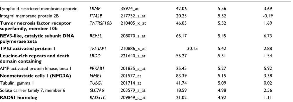
Verification of model predictions using small interfering RNA to p53
To validate the predictions made by the model, we transfected MOLT4 cells with small interfering (si)RNA to p53 to deplete p53 protein to below control levels (Figure 6a) [26]. siRNAp53 substantially reduced ionizing irradiation-induced increases in the transcripts of three p53 target genes, namely HDM2, P21, and GADD45α(Figure 6b). We then ran micro-arrays to measure the effect of siRNAp53 on the transcrip-tional response to irradiation at the whole genome level. Validation was carried out at 4 hours to maximize the number of p53 targets and to minimize the inclusion of secondary tar-gets. Data were filtered to identify those genes that were upregulated in both the time course and in the pSuper transfected control at 4 hours (see Materials and methods, below). This identified a total of 162 genes that were upregu-lated significantly by irradiation at 4 hours.
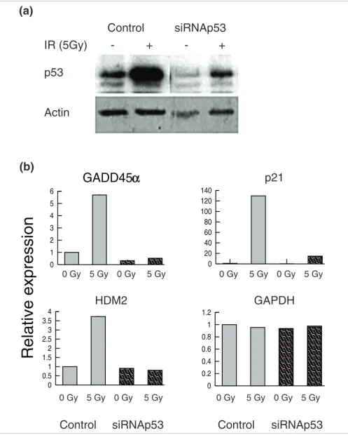
To quantify sensitivity to siRNAp53 at the individual gene level, we computed new Z scores that measured the difference between genes upregulated by irradiation in control cells and those upregulated in siRNAp53 treated cells. For clarity, these are referred to as validation scores. The higher the vali-dation score, the more effectively siRNAp53 eliminates change in transcript concentration, and so the more likely the gene is to be dependent on p53. Seventy-four of the 162 4-hour-upregulated genes were predicted by the model to be p53 targets because they fell into class 1 (M < 100 and sensi-tivity Z score > 2). Of these 74, 66 (90%) exhibited high (Z > 1) validation scores (namely sensitivity to siRNAp53), con-firming that they are p53 targets (Figure 7a). This figure rises to 73 out of 74 (98%) if a lower sensitivity Z score threshold (> 0.5) is applied or falls to 39 out of 74 (53%) if the sensitivity Z score threshold is set at 3. Higher sensitivity Z score thresh-olds therefore result in greater accuracy but at the expense of identifying a lower proportion of the targets (Figure 7b). Sen-sitivity Z score correlated well with validation score,
indicat-ing that predicted rank of p53 targets reflected the strength of p53 regulation (Figure 7c).
Thirty upregulated (4 hours) genes fell into class 2 (M > 100 and sensitivity Z score > 2). As expected, the response of class 2 genes to siRNAp53 was divided. Fourteen genes, including
TNFSF10 (TRAIL), remained unaffected by siRNAp53,
showing them to be p53 independent/irradiation dependent. Sixteen class 2 genes were affected to some degree by the treatment, confirming predictions that this group included co-activated or co-repressed genes such as IER3, which is known to be synergistically regulated by nuclear factor-κB and p53 [27]. The remaining 58 upregulated (4 hours) genes fell into class 3, 34 of which were affected by siRNAp53.
Overall the Z score for Sj (sensitivity to p53) was a good dis-criminator for identifying p53 targets. The model was able to predict with confidence, and at high accuracy, 66 out of 115 (57%) genes verified as p53 targets at 4 hours, based on a sen-sitivity Z score threshold of 2. A further 16 class 2 genes exhib-ited evidence of co-regulation, suggesting an explanation for 71% of the interpretable data. Many of the remaining class 3 targets were expressed at low levels, or exhibited low (> 1.5-fold) levels of differential expression. This raises questions about their biologic significance, and suggests that the true success rate of hidden variable dynamic modeling (HVDM) is actually higher than reported above. A larger number of rep-licates would be required to be confident of the status of class 3 genes.
As seen for the validation data set, tightening thresholds (by choosing a higher sensitivity Z score) results in more confi-dence that the targets are regulated by p53 but at the cost of explaining a lower percentage of the data (Figure 7). When applied to the entire upregulated data set, HVDM can accu-rately predict a large number of p53 targets from a short time course without any further experimental input (Figure 8). These predictions included a number of genes not previously known to be p53 targets, including CD38, DENN-domain protein FLJ22457, CROT, GLS2, HERC5, ASCC3, LRMP, and
Small interfering (si)RNAp53 reduces p53 protein levels and transcription of p53 target genes Figure 6 (see previous page)
Small interfering (si)RNAp53 reduces p53 protein levels and transcription of p53 target genes. (a) Transfection of siRNAp53 reduces p53 protein levels below control values. (b) Real-time quantitative polymerase chain reaction measurement of three p53 target genes (GADD45α, p21, and HDM2) and a control gene (GAPDH) after transfection of siRNAp53 and irradiation. IR, ionizing irradiation.
Model validation
Figure 7 (see following page)
Model validation. (a) Effect of small interfering (si)RNAp53 on irradiation (5 Gy) induced change in transcript levels at 4 hours of the 74 class 1 genes. (b) Effect of altering Sj Z score threshold for class 1 on proportion of true targets identified (% of p53 upregulated genes at 4 hours predicted; black line) and
Figure 7 (see legend on previous page)
0 2 4 6 8 10
5gy + 4 hours Unirradiated
Control
0 2 4 6 8 10
5gy + 4 hours Unirradiated
SiRNA p53
Normalised expression
-2
0
2
4
6
8
10
12
0
10
20
30
40
50
60
70
Validation score
(a)
(b)
(c)
Sensitivity Z score threshold
1
2
3
4
5
20
40
60
80
100
Percentage
Accuracy of prediction (%)
Proportion of targets identified (%)
comm
en
t
re
v
ie
w
s
re
ports
refer
e
e
d
re
sear
ch
de
p
o
si
te
d r
e
se
a
rch
interacti
o
ns
inf
o
rmation
CIKS/ACT1/TRAF3IP2 (Table 1). siRNA validation at an
early time point (4 hours) indicates that these genes are most likely to be direct targets. CD38 is best known as a prognostic marker in the leukemia B cell lymphocytic leukemia (B-CLL associated) with poor outcome. It functions as a powerful reg-ulator of calcium dependent signaling via the generation of cyclic ADP ribose and NAADP+ (nicotinic acid adenine dinu-cleotide phosphate) Its regulation by p53 suggests a possible role for calcium-dependent signaling in the DNA damage response.
Hidden variable dynamic modeling predicts p53 targets more accurately than does K means clustering Since both HVDM and clustering approaches aim to identify TF targets, we compared our results with a typical clustering approach, namely K means clustering. From the 754 genes identified as upregulated by irradiation, HVDM generated a ranked list of predicted p53 targets based on model score and best sensitivity Z scores (Table 1). Forty-eight of the 50 high-est ranked targets (96%) predicted by HVDM were confirmed by siRNA to be p53 targets. These 50 HVDM predicted target genes were divided by K means clustering between six of eight clusters, each with a distinct response profile (Figure 9). For example, the HVDM predicted target TP53TG1 has a late expression profile (cluster 1, Figure 9), along with seven other top 50 targets. This profile is quite different from the activa-tion profile of p53 or its 'typical' correlated targets (Figure 5b). Only two genes were probably false positives.
K means clustering of the 754 detected and upregulated genes based on expression levels alone grouped the genes into eight clusters based on transcript time profile (Figure 9). Visual examination of the profiles suggested that one of these classes
(cluster 7, Figure 9) was most similar to the p53 activity pro-file determined by Western blot (Figure 5b), and indeed this cluster contained many of the well known p53 targets
(includ-ing GADD45α, p21, and DDB2). However, because clustering
approaches typically do not provide confidence intervals, it is impossible to identify which genes within the cluster are most or least likely to be real targets. We found that 25 out of 79 genes in cluster 7 were verified as p53 targets in the siRNA experiment (32%; data not shown). Verified genes also occurred in cluster 1 (11 out of 135 (8%)), cluster 3 (35 out of 102 (34%)), cluster 4 (21 out of 120 (17.5%)), cluster 5 (3 out of 90 (3.3%)), and cluster 6 (20 out of 51 (39%)).
In summary, HVDM can generate an accurate list of p53 tar-gets with different expression profiles, ranked by probability of sensitivity to p53. In contrast, although K means clustering generates clusters enriched or depleted in p53 targets, it fails to identify targets with different profiles, is unable to quantify the level of sensitivity of a gene to p53, and cannot distinguish between true and false p53 targets. We also assessed the per-formance of self-organizing maps (SOM) clustering, with a similar outcome. This is expected, given that all processes that cluster on expression profile alone are bound to suffer similar deficiencies. Predictions made by HVDM are there-fore accurate, explain a significant proportion of true targets, give indications about potential for co-regulation, and provide an excellent basis for prioritization of downstream bioinformatics and experimental analysis.
Discussion
We present here an approach based on a simple differential equation model that uses hidden information to partially reconstruct, with confidence intervals, the p53 target net-work. Our algorithm, which we term hidden variable dynamic modeling, operates on two levels. First, it offers a quantitative description of a TF output network at the genomic level. Second, it provides a practical resource to enable the predic-tion of targets and a probability based prioritizapredic-tion of array data for downstream analysis.
Mathematical modeling of gene networks has taken a variety of approaches [3,11,12]. At the genome level, topographic network reconstruction has been achieved using a variety of methods and data sources, including microarray data [1,28-30]. In contrast, dynamic modeling has typically been limited to short pathways or feedback loops because of the complex-ity associated with estimating high dimensional models [11]. Some attempts to group network behavior into modules for dynamic modeling have been successful [13]. Others have attempted dynamic modeling of whole microarray data sets using differential equation models to derive transcriptional profiles [5,6,31]. However, these interesting studies stop short of calculating confidence intervals that take into account measurement error and variability [31,32]. Without these measurements, the reliability of the model cannot be
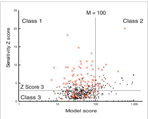
[image:11.612.54.296.85.280.2]Model performance Figure 8
Model performance. Distribution of 459 upregulated genes that pass degradation filter based on model score and predicted sensitivity to p53. Sj
Z score = 3 and model = 100 thresholds are shown. A total of 115 Genes verified as p53 targets at 4 hours are shown in red.
0 5 10 15 20 25
1 10 100 1,000
er
o
c
s
Z
yti
vit
is
n
e
S
Model score Z Score 3
Class 3
M = 100
K means clustering of upregulated genes based on expression values Figure 9
K means clustering of upregulated genes based on expression values. A total of 754 upregulated genes were optimally grouped into eight K means clusters (C1 to C8). The 50 best hidden variable dynamic modeling predictions (Table 1) are split among six clusters (highlighted in yellow). Accurate prediction of p53 targets is therefore not possible using K means at this level.
C1
C4
C7
C5
C2
C3
C8
Time (h)
Log (nor
malised e
xpression)
comm
en
t
re
v
ie
w
s
re
ports
refer
e
e
d
re
sear
ch
de
p
o
si
te
d r
e
se
a
rch
interacti
o
ns
inf
o
rmation
assessed. Neither do they test predictions made by the model by experimentation.
Most microarray data are analyzed by subjecting them to var-ious levels of statistical filtering to identify differences between two or more conditions. The resultant list of genes may then be segregated according to gene ontology using var-ious tools designed for this purpose [33]. It is assumed that co-regulation of genes with a particular ontology is of interest, but this may be misleading and certainly cannot predict tar-gets of a particular TF. Correlation approaches that cluster genes that exhibit a similar time course expression profile are more successful [34], but they are often inaccurate and miss many genuine targets with a different profile. The advantage of our approach is that it can predict genes with any profile as targets of the same TF.
Complex data sets contain hidden information about gene regulatory networks [35]. It has also been suggested that the use of prior biologic knowledge can improve the reconstruc-tion of genetic networks [36]. In generating our model, we used a small amount of knowledge about TF targets to derive the activity profile of p53 and then applied this to partially reconstruct the p53 target network. Our model makes the assumption that, given a short time course, much of the net-work behavior can be explained using linear modeling, and our verification experiment strongly supports this assertion (Table 1). However, it is likely that some genes respond to p53 in a nonlinear manner, for instance as a result of saturation and/or threshold effects. Future extensions of our model to include these terms may explain an even higher proportion of the behavior (work in progress). It should also be noted that the model would be unable to distinguish between TFs with identical activity profiles. Combination of HVDM with exper-imental approaches or other in silico methods such as the identification of TF-binding sites could help to resolve this issue [37-39]. The current model is only able to account for direct effects of the controlling TF, which is reasonable for the short time course employed in our studies. Future modifica-tions to the model will permit modeling of secondary effects, namely genes upregulated at late time points that may be tar-gets of tartar-gets.
HVDM correctly predicted the majority of p53 targets, includ-ing all of the well known examples, directly from time series measurements of a complex response. HVDM was also able to identify, with associated probability, genes that had not pre-viously been identified as p53 targets. Several previous studies have aimed to identify p53 target genes on a genome wide level using microarrays. Zhao and coworkers [22] iden-tified p53 targets by using a Zn2+-inducible p53 construct
containing a metallothionein promoter. In this case, the spe-cific induction of p53 required the establishment of a complex and artificial in vivo system. p53 targets could not be directly extracted from ionizing irradiation or ultraviolet irradiation experiments alone. Also, targets induced in the artificial
sys-tem differed significantly from those induced by ionizing irra-diation or ultraviolet, indicating that simple artificial systems cannot replicate the behavior of complex activities during a physiologic response. In another approach, Kannan and cow-orkers [40] employed a temperature sensitive p53 to identify p53 dependent transcription and used cycloheximide to dis-tinguish between primary and secondary targets. However, again, a complex artificial system was required. Furthermore, temperature and cycloheximide are both likely to affect the resultant transcription patterns, and because the data cannot be ranked the reliability of many targets would require additional experimental verification. HVDM has the advan-tage that ranked probability based target lists can be extracted from complex data without having to isolate each factor experimentally.
We observed that genes that were affected by siRNAp53 but not predicted by the model typically exhibited expression lev-els close to the detection threshold or low levlev-els of differential regulation, or were poorly hybridizing alternative probe sets for genes already predicted by the model to be targets. The biologic significance of many apparent targets not identified by the model is therefore questionable. The ability to provide ranked lists of predicted (class 1) targets with a high degree of confidence, and based on the minimum of input data, will allow researchers to make optimal use of their resources. Such prioritization has been lacking in microarray data anal-ysis and has hampered the efficient interpretation of array experiments.
It is important to note that the model is dynamic. It not only identifies targets but also predicts network behavior in response to changing conditions or altered parameters. For example, treatment with a drug that alters p53 activity could potentially be modeled entirely in silico based on its effects on expression of the training set of target genes. This may have implications for predicting the consequence of clinical or experimental treatments [41].
Conclusion
We addressed the problem of extracting hidden information from time series microarray data. We present a method that models the p53 target network following DNA damage, in which we use prior biologic information (a training set) to construct a mathematical model of the transcriptional response to DNA damage in MOLT4 cells. We have also developed a method to calculate confidence intervals for parameter estimates in a highly efficient manner. We found that the inclusion of a surprisingly small amount of additional biologic information was necessary to anchor the model. Most importantly, we then successfully tested the model pre-dictions with an entirely separate experimental data set.
The model identified genes not previously known to be p53 regulated, and it is more widely applicable and more accurate than correlation or clustering methods because it considers degradation rates as well as transcript accumulation profiles. Furthermore, HVDM can extract hidden information from small data sets in which experimental methods would require an impractical number of observations. Finally, HVDM allows the probability-based prioritization of microarray data, permitting researchers to exclude irrelevant informa-tion and rapidly focus on the networks of interest.
HVDM can be applied to any large time series data set in which identification of hidden variables can reveal critical information about network dynamics. The approach is quan-titative and predictive, and demonstrates that combining mathematical modeling with experimental observations can help to unravel complex relationships in biologic systems.
Materials and methods
Biological methodsCell lines and reagents
Human MOLT4 cells (T cell acute lymphoblastic leukaemia) were obtained from the National Institute for Biological Standards and Controls (Potters Bar, Herts, K; CFARP011) and cultured in RPMI, 10% fetal calf serum and L-glutamine, plus antibiotics. p53 genotype was determined by sequencing to verify wild-type status. p53 accumulation was monitored after irradiation by quantitative Western blotting, and regula-tion of known p53 targets (p21, GADD45α, and MDM2) fol-lowing p53 activation by ionizing radiation was established to confirm p53 wild-type behavior (data not shown). Western blots were probed against total p53 (Santa Cruz Biotechnol-ogy Inc. Santa Cruz, CA, USA), phospho-p53 (Cell Signalling Technologies, Danvers, MA, USA), and actin (Santa Cruz). Proteins were detected using enhanced chemiluminescence (ECL+; GE Healthcare, Chalfont St Giles, Bucks, UK) and quantified by densitometry.
Microarray time course
Cells in log phase (1 × 10⁶/ml) were γ-irradiated with 5 Gy at
room temperature at a dose rate of 2.45 Gy/minute with a
137Cs γ-irradiator. Cells were harvested at 0, 2, 4, 6, 8, 10 and
12 hours, and RNA and protein were extracted (Trizol; Invit-rogen, Paisley, UK). RNA and cRNA quantity and quality were determined by Nanodrop spectophotometer and Bioan-alyser 2100 (Agilent, Wokingham, Berks, UK). Affymetrix U133A arrays (Affymetrix, Sanat Clara, CA, USA) were hybridized as standard. Array quality was determined using R and GCOS .rpt file values. The time course was replicated three times from independent cell preparations.
Microarray data analysis
Microarray data were summarized using the MAS5.0 algo-rithm (Affymetrix). Signal distribution was assessed using Genespring 6.1 (Agilent), and data were normalised to the
median and log transformed for further analysis. For mode-ling applications, rescaled MAS5.0 data were analyzed using C code [42] (see Mathematical methodology, below). Data are available in MAGE-ML format via ArrayExpress (European Bioinformatics Institute) or on request.
Prediction of p53 targets
Data were filtered to identify 754 genes that were confidently upregulated by ionizing radiation (but not necessarily by p53) in at least one time point, and to exclude control genes (for example, spike ins). We excluded genes predicted to have a biologically impossible degradation rate (either close to zero (< 0.01/hour) or with too short a half-life (rate > 5/hour)). Next, we calculated the sum M of weighted differences between the model predicted profile and the experimentally determined transcript profile. Finally, the confidence that the transcript was sensitive to p53 activation was assessed by determining the probability that each individual sensitivity Sj was equal to 0. The modeling and statistical techniques used to compute these indicators are described extensively below.
Real-time quantitative polymerase chain reaction
MOLT4 cells were irradiated with 5 Gy and incubated at 37°C for various time periods. First strand cDNA was prepared (Invitrogen) and used as a template in PCR reactions with predeveloped target assays (Applied Biosystems, Foster City, CA, USA): p21, HDM2, GADD45, and GAPDH. Target and reference were amplified in separate wells in a 96-well setup with three replicates for each reaction on ABI Prism SDS 7000 (Applied Biosystems), using default cycling conditions. Change in gene expression was calculated using 2-dCT, where
dCT is the mean of CT (threshold cycle number) values obtained from the triplicate samples at each time point.
Small interfering RNA experiments
comm
en
t
re
v
ie
w
s
re
ports
refer
e
e
d
re
sear
ch
de
p
o
si
te
d r
e
se
a
rch
interacti
o
ns
inf
o
rmation
Mathematical methods
Model formulation
We assume that the transcript concentration xj(t) of gene j satisfies the following time-dependent linear differential equation:
This assumes that the transcript is degraded proportionally to its concentration, with the degradation rate Dj. The produc-tion term Bj + Sjf(t) comprises a basal transcription rate Bj, which may be increased proportionally by the TF activity f(t). Sj is the sensitivity of gene j to that TF. Our overall aim is to estimate the parameters Bj, Sj, and Dj from the microarray
data [ j(ti)], and in particular the sensitivity Sj. If Sj is not sig-nificantly greater than zero, then gene j is not regulated by the TF, whereas if Sj is large and significantly different from zero then the TF has a very strong effect on that gene.
The activity level f(t) of the TF (p53) is unknown. In order to estimate the hidden variable f(t), we need to parametrize the function f and estimate the resulting parameters. This raises the problem that if we try to estimate the unknown parame-ters in Equation 1 for single gene j, then we have more unknown parameters than we have data points. The unknowns are the three parameters Bj, Sj, Dj, and the n + 1 values f(t0) ... f(tn), as compared to the n + 1 observed data
points j(t0) ... j(tn). (The term j is the experimental measurements of gene j, composed of xj + ε, where ε is the measurement error.)
We observed that the equations for different genes are cou-pled by the level f(t) of the TF. Thus if we measure m genes simultaneously with microarrays, then we have m(n + 1)
measurements j(ti) for j = 1 ... m and i = 0 ... n, but there are only 3 m + n + 1 unknowns Bj, Sj, Dj for j = 1 ... m and f(t0) ... f(tn). If the number of time points n is sufficiently large, then m(n + 1) = 3 m + n + 1, and we are able to estimate the unknowns using standard optimization methods. In practice we applied the model to replicate measurements that requires a modification to this approach (see Additional data file 1).
As the model stands, different parameter combinations could give rise to identical solutions for xj(t). This is because both the origin and the scaling of the unobserved TF activity are
arbitrary. Suppose that f(t) = α (t) + β for some constants α ≠ 0 and β. Then Equation 1 becomes the following:
Where j = Bj + Sjβ and = αSj. Because the TF is not observed, we have no way to distinguish between the models in Equation 1 and Equation 2. To overcome this ambiguity, we first set Sj = 1 for one gene, in our case p21. This fixes α and removes the ambiguity from the remaining Sj and reduces by one the total number of parameters to be estimated. Second, we assume that at the start of the experiment the activity level of the TF is 0. In other words, we set f(t0) = 0, which is suffi-cient to fix β and hence remove the ambiguity from the Bj. It further reduces the parameter count by one.
Setting f(t0) = 0 has the effect of defining the basal transcrip-tion rate Bj for each gene as the rate at the start of the experi-ment. We assume that the p53 network is in equilibrium before irradiation, and hence Bj can be thought of as the equilibrium transcription rate. Similarly, f can be interpreted as the deviation from equilibrium of the transcription factor activity.
Discretizing the model
In a systems biology context it is necessary to screen thou-sands of potential targets. We therefore developed a very rapid numerical method for estimating parameters in Equa-tion 1.
Since Equation 1 is linear, it is possible to obtain an analytic solution:
We found that parameter estimation by direct application of standard numerical schemes for the evaluation of integrals was too slow. These approaches also suffer from the require-ment to define an appropriate functional form and parametri-zation of f(t).
Instead, motivated by collocation based approaches to boundary value problems for nonlinear differential equa-tions, we chose to discretize the model directly, converting the problem into an algebraic one. We illustrate this approach using the simplest possible discretization scheme.
To estimate the parameters in Equation 1 we must evaluate the derivative, which we denote ∆i, on the left hand side at a
specific time point ti. Knowing the values xj(ti-1), xj(ti), and xj(ti+1) at neighboring points, we computed the slope of xj(t) between ti-1 and ti, and the slope between ti and ti+1. We then dx t
dt B S f t D x t
j
j j j j
( )
( ) ( )
= + −
( )
1˘
x
˘
x ˘x ˘x
˘
x
f
dx t
dt B S f t D x t
B S S f t D x t
j
j j j j
j j j j j
( )
( ( ) ) ( )
( ) ( ) ( )
= + + −
= + + −
α β
β α
== + −
( )
Bj S f tj ( ) D x tj j( )
2
B S
x t B
D e S f t e dt
j j
j D t
j D t
t
j j
combined these two values using an appropriate weighting and obtained an estimate for ∆i (for notational convenience
we define xi = xj(ti-1)). If the time intervals are regular, so that ti - ti-1 = ti+1 - ti, then:
This is equivalent to fitting a quadratic polynomial to the three points, and then evaluating its derivative at ti. Higher order approximations can be obtained by using more points and fitting an appropriate polynomial. A suitable way of doing this is Lagrange interpolation [42]. This gives an explicit formula for a degree q - 1 polynomial P(t) passing through the q points (tp, xp) ... (ti, xi) ... (tr, xr), where r = p + q - 1:
Where
We call such an approximation a q-point approximation (so that the example above gives a three-point approximation). An approximation of the required derivative ∆i can now be
obtained by differentiating P(t) at ti.
The right hand side is a linear function of x0 ... xn. We shall denote the coefficients of this by Aik, so that:
Where we set Aik = 0 for k < p or k > r. (For a detailed calcula-tion of Aik, see Additional data file 1.) We can then collate these various coefficients into a (n + 1) × (n + 1) matrix A. If we define the (n + 1) vectors as follows:
xj = [xj(t0) ... xj(tn)] = (x0 ... xn)
f = [f(t0) ... f(tn)] = (f0 ... fn)
1 = (1 ... 1)
Then our approximation of Equation 1 can then be written as follows:
Axj = Bj1 + Sjf - Djxj (6)
The formal solution is given by
xj = (A + DjI)-1(Bj1 + Sjf)
Where I is the (n + 1) × (n + 1) identity matrix. In practice we solve Equation 6 using the Loewr-Upper decomposition [42] of (A + DjI).
Our approach to the solution of Equation 1 is several orders of magnitude faster than a naïve approach to solving the differ-ential equation using an explicit fourth order Runge-Kutta, with the typical step size that would be employed in such a case. It also has the advantage that it is not necessary to spec-ify a functional form for f(t). In our case f(t) is simply repre-sented by the discrete set of values (f0 ... fn), that is by the vector f.
Although our approach implicitly integrates the differential equation using large step sizes (effectively ti+1 - ti), the una-voidable errors associated with estimating f(t) swamp any advantage gained by using smaller steps, and consequently there is no loss of accuracy in replacing Equation 1 by Equa-tion 6. We validated this conclusion by generating artificial data and adding Gaussian noise of similar amplitude to that generally seen in microarray data. We found that the error in the parameter estimation induced by this noise overshadows the discretization error.
Model fitting
We employed the discretized model described in Equation 6 in two different ways. First, to estimate the TF profile f(t), we fit a microarray time series to a training set of five genes known to depend on p53 (DDB2, p21WAF1/CIP1, SESN1/hPA26, BIK, and TNFRSF10b/TRAILreceptor 2). In order to do this, we also needed to estimate the parameters Bj, Sj, and Dj for these genes, although the estimated values are of no direct interest. We call the estimated profile obtained from this
phase = ( 0 ... n). We then used the estimated profile
and applied the model to the transcription time series [ j(t0)
... j(tn)] for each gene j in our data set to estimate Bj, Sj, and Dj.
In each phase we employed a standard approach to fitting the unknown parameters. We define a candidate parameter vec-tor, which in the first phase is given by the following equation:
µ = (B1 ... Bm, S1 ... Sm, D1 ... Dm, f0 ... fn)
In the second phase it is given by:
µj = (Bj, Sj, Dj)
Equation 6 was solved for this set of parameters using the LU decomposition of (A + DjI). In the first phase f = (f0 ... fn), with the fi taken from the candidate parameter vector µ. In the
∆i i i
i i
x x
t t
≈ −
−
+ −
+ −
1 1
1 1
P t C k p r t xk
k p r
( )= ( , , , )
( )
=
∑
3C(k, p, r, t)= t
t j
k r
j=p j k
−
−
( )
≠
∏
ttj 4∆ ≈i =
∑
i k=p i k
r d
dtP(t)t=t
d
dtC(k,p,r,t)t=t X
∆ ≈
( )
=
∑
i A Xik k
k n
0
5 ,
f f f f
˘
x
˘
comm en t re v ie w s re ports refer e e d re sear ch de p o si te d r e se a rch interacti o ns inf o rmation
second phase we used = ( 1 ... m) obtained from the first phase. We then computed the error Mj (depending on µ or µj,
respectively) for each gene between the model solution and the actual data:
We assume the measurement errors to be independent and normally distributed with standard deviation σj(ti) for the
observation at time ti of gene j. The calculation of σj(ti) is detailed in Additional data file 1.
In the first phase the error over the training set (containing m genes) is then
To fit the model, we then varied µ or µj in a systematic way to
find the parameters that make M or Mj as small as possible using a MCMC method [23]. This has the added advantage of also providing confidence intervals for the resulting parame-ter estimates. We assume that the measurement errors are Gaussian, giving a likelihood function proportional to exp (-M/2) or exp(-Mj/2). A Metropolis-Gibbs sampler was then applied with this likelihood. Because neither Bj nor Dj can take negative values, the MCMC sampling was carried out in logarithmic space for these two parameters [(og(Bj) and log(Dj), respectively).
To improve the convergence speed of the MCMC scheme it is advantageous to make jumps in the parameter space that are commensurate with the different parameter scales. This is particularly the case in the first phase, in which the dimen-sionality of the parameter space is high. We estimated such scales by running partial MCMC schemes on each group of parameters in turn, before running the full MCMC scheme. Specifically, parameters were grouped into four sets: degra-dation, transcription, basal rates, and TF profile. For each set a scale was determined to achieve an acceptance rate of approximately 25%. A final tuning run was carried out on the whole parameter set in order to achieve the prescribed acceptance rate of 25%. The main MCMC was seeded with the minimum of M found from a standard optimization proce-dure (the Nelder-Mead simplex algorithm). A burn in of 10,000 iterations was applied before proper sampling. The final sample of 10,000 observations was extracted at random from the 107 iterations following burn in. We verified that
these choices yielded good convergence.
In the second phase, in which the TF profile is known and there are only three parameters to determine, a long iteration run is unnecessary. We found that 105 iterations were
suffi-cient to produce good convergence. Once again 10,000 obser-vations randomly sampled from those iterations were used to compute the relevant statistics.
Additional data files
The following additional data are included with the online version of this article: A Word document giving details of the rescaling of array data, derivation of the coefficients of the differential operator, extension of model fitting to replicate measurements, and estimation of the measurement error (Additional data file 1).
Additional data file 1
A Word document giving details of the rescaling of array data A Word document giving details of the rescaling of array data, der-ivation of the coefficients of the differential operator, extension of model fitting to replicate measurements, and estimation of the measurement error
Click here for file
Acknowledgements
The ARP011 MOLT4 cell line was provided by NIBSC/CFAR through the EU Programme EVA/MRC Centralised Facility for AIDS Reagents, UK (grant Number QLK2-CT-1999-00609 and GP 828102). MB and DT are supported by postdoctoral fellowships from the BBSRC. DB holds a CHRAT studentship at ICH. We thank Lola Martinez for FACS sorting and Nipurna Jina for assistance with microarrays. This work was funded by the BBSRC as part of the Exploiting Genomics initiative.
References
1. Gardner TS, di Bernardo D, Lorenz D, Collins JJ: Inferring genetic networks and identifying compound mode of action via expression profiling. Science 2003, 301:102-105.
2. Sontag E, Kiyatkin A, Kholodenko BN: Inferring dynamic archi-tecture of cellular networks using time series of gene expres-sion, protein and metabolite data. Bioinformatics 2004, 20:1877-1886.
3. Stark J, Brewer D, Barenco M, Tomescu D, Callard R, Hubank M: Reconstructing gene networks: what are the limits? Biochem Soc Trans 2003, 31:1519-1525.
4. Ronen M, Rosenberg R, Shraiman BI, Alon U: Assigning numbers to the arrows: parameterizing a gene regulation network by using accurate expression kinetics. Proc Natl Acad Sci USA 2002, 99:10555-10560.
5. Chen HC, Lee HC, Lin TY, Li WH, Chen BS: Quantitative charac-terization of the transcriptional regulatory network in the yeast cell cycle. Bioinformatics 2004, 20:1914-1927.
6. Chang WC, Li CW, Chen BS: Quantitative inference of dynamic regulatory pathways via microarray data. BMC Bioinformatics 2005, 6:44.
7. Lee TI, Rinaldi NJ, Robert F, Odom DT, Bar-Joseph Z, Gerber GK, Hannett NM, Harbison CT, Thompson CM, Simon I, et al.: Tran-scriptional regulatory networks in Saccharomyces cerevisiae. Science 2002, 298:799-804.
8. Mukherjee S, Berger MF, Jona G, Wang XS, Muzzey D, Snyder M, Young RA, Bulyk ML: Rapid analysis of the DNA-binding specif-icities of transcription factors with DNA microarrays. Nat Genet 2004, 36:1331-1339.
9. Harbison CT, Gordon DB, Lee TI, Rinaldi NJ, Macisaac KD, Danford TW, Hannett NM, Tagne JB, Reynolds DB, Yoo J, et al.: Transcrip-tional regulatory code of a eukaryotic genome. Nature 2004, 431:99-104.
10. Hall DA, Zhu H, Zhu X, Royce T, Gerstein M, Snyder M: Regulation of gene expression by a metabolic enzyme. Science 2004, 306:482-484.
11. Stark J, Callard R, Hubank M: From the top down: towards a pre-dictive biology of signalling networks. Trends Biotechnol 2003, 21:290-293.
12. Schlitt T, Brazma A: Modelling gene networks at different organisational levels. FEBS Lett 2005, 579:1859-1866.
13. Kholodenko BN, Kiyatkin A, Bruggeman FJ, Sontag E, Westerhoff HV, Hoek JB: Untangling the wires: a strategy to trace functional interactions in signaling and gene networks. Proc Natl Acad Sci USA 2002, 99:12841-12846.
14. Fei P, El-Deiry WS: P53 and radiation responses. Oncogene 2003, 22:5774-5783.
f f f
M x t x t
t )
j j i j i
j i i=0 n = −
( )
∑
( )σ ( ˘( )2
7
M= Mj
j=1 m