Munich Personal RePEc Archive
Are eBay auctions efficient? A model
with buyer entries
Huang, Ching-I
National Taiwan University
14 March 2008
Online at
https://mpra.ub.uni-muenchen.de/7754/
Are eBay Auctions Efficient? A Model with Buyer Entries
Ching-I Huang∗
March 14, 2008
Abstract
I use a sequential-auction model to mimic the environment of Internet auction sites,
such as eBay. For a sequence of auctions, new buyers may enter the auction site after
some of the auctions has completed and only bid for the remaining auctions. Because an
incumbent buyer may have revealed their own valuation in earlier auctions while a new
entrant do not, their expectations about the future are asymmetric. As a result, a buyer
with a lower valuation may win an auction while a buyer with a higher valuation may
restrain from bidding higher, resulting an inefficient allocation. On the contrary, selling
the multiple items in a single simultaneous auction results in an efficient outcome. The
profit from selling all items together in one simultaneous auction is less than that from
selling them sequentially.
1
Introduction
Internet auctions have grown rapidly in the past decade. Although there have been many
researches focusing on Internet auctions1, one important feature of Internet auctions remain
lack of attention. Contrary to most traditional brick-and-mortar auctions, buyers do not
arrive at an Internet auction site simultaneously. For a sequence of auctions, new buyers may
enter the auction site only later in the sequence.
∗Department of Economics, National Taiwan University, Taipei, Taiwan. I would like to thank Joseph
Taoyi Wang and Jong-Rong Chen for helpful comments and discussions. Financial supports from the National Science Council in Taiwan are gratefully acknowledged. All remaining errors are mine.
In the tradition models of sequential auctions, all buyers arrive before the first auction
takes place. (See, for example, Weber (1983); Milgrom and Weber (2000).) An auction begins
after the previous one has completed. If a buyer does not win in the previous auction, she
can participate in the next one. Because of the future options, buyers would lower their
bids in the previous auction. With independent privatevalues, Weber (1983) shows that the
expected price of each auction is the same for both the sequential first-price and
second-price auctions because the effect of winners leaving the auction site and the effect of bidders
shading their bids in early auctions to account for future options cancel out. Huang, Chen,
Chen, and Chow (2008) propose a model to analyze Internet auctions with buyer entry. They
find parallel auctions can be viewed as sequentially auctions because buyers only bid on the
auction which is the first one to end among all remaining auctions. The allocation is efficient
even when entry is possible. Nonetheless, they only analyze independent private valuations
among buyers. In this paper, I find that the efficiency does not hold if valuations are allowed
to be affiliated.
When buyers’ valuations are affiliated, the analysis is much more complicated. There is
still no complete answer for a fully general auction model. Milgrom and Weber (2000) find
that sequential first-price auctions would have ascending expected prices because buyers are
willing to bid more in later auctions after observing the information revealed in earlier
auc-tions. As for sequential second-price auctions, Wang (2006) shows that the expected prices
also ascend in a sequential second-price auction with affiliated private values. Zeithammer
(2006) extends the model of sequential auctions from selling identical items to selling
het-erogenous items. Contrary to the theoretical findings about affiliated value auctions, empirical
studies tend to find descending prices across auctions.2
The model in this paper consists of a sequence of ascending auctions. Each of them sells an
identical good. All buyers have inelastic unit demand for the good. Buyers enter the auction
site sequentially and stay until winning a good. I characterize a perfect Bayesian equilibrium
in this game. An important result of this paper is that the allocation of the auction mechanism
is not necessarily efficient. It is possible that a buyer with a lower valuation obtains the good
while a buyer with a higher valuation does not. Allowing new buyers to enter per se does
not necessarily result in inefficiency in the allocation of the items. However, when buyers’
valuations are affiliated, inefficiency results from the information asymmetry among buyers.
The driving force behind the the inefficiency is the asymmetry of buyers. While some
buyers participate in an earlier auction and reveal their own valuations to all other buyers
by submitting bids, new buyers do not. Since new buyers also know their own private
val-uations, they have better information than old buyers. Because of affiliation in valval-uations,
the asymmetry in turn creates different expectations about the valuations of future incoming
buyers. New buyers get information rents from their better information and bid less
aggres-sively, other things being equal. Hence, the allocation of the sequential auctions is not always
efficient.
I also find transaction prices to be identical across auctions in the sequential auction model
considered in this paper. This price is higher than the price of selling all the items together
in a single multiple-object auction. Consequently, in order to maximize the expected profit,
a seller with several identical items to sell should offer them in a sequence of single-object
auctions rather than in one multiple-object simultaneous auction.
The inefficiency remains possible if sequential ascending auctions are replaced by
sequen-tial sealed-bid second-price auctions. Information asymmetry is still a reason for inefficiency.
Nonetheless, in addition to selling the good to the less informed buyer when she has a lower
valuation, efficiency may also occur in the opposition case, selling the good to the more
informed buyer when she has a lower valuation.
The rest of the paper is organized as the following. In the next section, I introduce a model
which mimics sequential eBay auctions with buyer entries. A perfect Baysian equilibrium is
presented in Section 3. In Section 4, I compare the eBay type auction with other formats of
auctions. To provide a concrete idea of the model equilibrium, I show an numerical example
2
Model
Consider an affiliated private value model with three auctions and four buyers. Under the
private value assumption, each buyer has perfect information about her own valuation for
the item. Under the affiliatedvalue assumption, buyers’ valuations are positively correlated.
When there are only two auctions, the information obtained in the first auction is useless in
the second auction because it is a dominant strategy to bid one’s own valuation in the second
(final) auction. The simplest model to show the effect of asymmetric information is to have
three auctions and four buyers. The model can be extended to have more auctions without
changing the result of the information asymmetry among buyers.
Following the empirical findings in Zeithammer and Adams (2006), I model eBay auctions
as ascending auctions.3 Assume that three auctions, each with one identical object to be sold,
will be held sequentially in periodst= 1,2,3, respectively.4
One buyer enters in each period t= 0,1,2,3. Let the random variable Vi represent the
valuation of the buyer who enters in period i−1, i= 1,2,3,4. The realized value of Vi is
denoted as vi. While the joint distribution of (V1, V2, V3, V4) is common knowledge among all buyers, the realized valuevi is not. The valuations Vi are affiliated in the sense that the
conditional expectation E[Vi|V−i = v−i] increases in each components of v−i, where v−i ≡
(v1, . . . , v−i, vi+1, . . . , v4). The distribution function of (V1, V2, V3, V4) is non-degenerate. The support of eachViis an interval [v, v]. To simplify the exposition, assume the joint distribution
of V1 and V2 are symmetric. Every buyer is risk-neutral and demands only one object. It is costless to bid. There is no discount between periods. A buyer’s surplus is her valuation vi
less the transaction price if she wins in one of the auctions. The surplus is zero otherwise. A
buyer wants to maximize her surplus. Since all buyers has inelastic unit demand, a winning
bidder will not participate in future auctions.
Auctions are conducted as a “button auction” in each period. All buyers press on a
3They empirically test the bidding behavior on eBay and find the data are better described by ascending
auctions rather than second-price sealed-bid auctions.
button at the beginning of a period. The standing price starts from v and keeps rising. A buyer depresses the button once she decides to quit from the current auction. When a buyer
quits from one auction, she cannot re-enter the same auction. The standing price rises until
only one buyer left. The last remaining buyer wins the auction and pays the final standing
price. The final standing price is announced to all buyer, including future buyers.
Since buyers’ valuations are random variables, the transaction prices are also random
variables. LetP∗
t denote the transaction price of the auction in periodt. Its realized value is
represented by the lowercase p∗
t.
3
Perfect Bayesian Equilibrium
In this section, I will derive a perfect Baysian equilibrium of this three-period auction game
by backward induction. Because the joint distribution of (V1, V2) is symmetric, without loss of generality, I only need to consider subgames after the histories with V1 ≥ V2. For the subgames after the histories V1 ≤ V2, I simply need to exchange the scripts 1 and 2 in the analysis. Therefore, I will assume V1 ≥V2 for the rest of the paper.
3.1 The Final Auction
As is well-known in the literature, a buyer’s dominant strategy in a second-price ascending
auction is to bid until her own valuation. The bidding strategy of a buyer with valuationv in the final auction is to bid until the price rises to her own valuation, β3(v) =v. This strategy is independent of information. As a result, the winner of Auction 3 is the buyer with the
higher valuation in this period. The transaction price equals to the lower valuation among
the two buyers.
3.2 The Second Auction
Consider the history after the buyer with the higher valuation in period one has won the first
the dominant strategy in the final auction is to bid until a buyer’s own valuation, regardless
of other buyers’ valuations. There is no strategic concern in the second auction to conceal
one’s own valuation.
Suppose the bidding strategy in the first auction is a strictly increasing function of a
buyer’s valuation. Then the realized valuation v2 can be inferred from the transaction price of Auction 1, p∗
1, and the bidding function for the first auction β1. Denote the inferred value of Buyer 2’s valuation by ˆv2 = β1−1(p∗1), it is public information in this period. In the equilibrium path, ˆv2 =v2. On the contrary, the new buyer’s valuation v3 is her private information. The two buyers process different information sets. Consequently, they would
have different expectations on the valuation about the future entrant,V4, which in turn affect their bidding strategies.
Let Sn
2(v3; ˆv2) be the newbuyer’s expected surplus of participating in the next auction, where v3 is her own valuation and ˆv2 is the inferred value of her opponent’s valuation. Note that the current standing pricep2 does not enter the expected payoff on the equilibrium path because there is no information gain from observing the price.
S2n(v3; ˆv2) =
Z v3
v
(v3−v4)dF4(v4|V2 = ˆv2, V3 =v3)
=
Z v3
v
F4(v4|V2 = ˆv2, V3 =v3)dv4. (1)
Buyer 3’s expected surplus depends on Buyer 2’s valuation ˆv2 because her surplus depends on the distribution of Buyer 4’s valuation, which is affiliated withV2.
The following lemma shows Buyer 3’s bidding strategy for the second auction.
Lemma 1. Buyer 3 keeps bidding on Auction 2 until the payoff from the Auction 2 is just
indifferent to the expected future payoff, v3−p2 =S2n(v3; ˆv2).
if and only if p2 ≤p∗. Buyer 3 prefers Auction 2 over Auction 3 if and only if p2 < p∗.
The maximal amount Buyer 3 is willing to bid on Auction 2 can be denoted as
β2n(v3; ˆv2) =v3−Sn2(v3; ˆv2). (2)
Lemma 2. βn
2(v3; ˆv2) is strictly increasing inv3 for any givenvˆ2.
Proof. For anyv′
3> v3,
βn
2(v3′; ˆv2)−β2n(v3; ˆv2) =−
Z v3
v
F4(v4|V2= ˆv2, V3=v′3)−F4(v4|V2 = ˆv2, V3=v3)dv4
+
Z v′3
v3
1−F4(v4|V2= ˆv2, V3 =v3′)
dv4.
Because V3 and V4 are affiliated, F4(v4|V2 = ˆv2, V3 = v′3) ≤ F4(v4|V2 = ˆv2, V3 = v3) for all
v4. In addition, F4(v3|V2 =v2, V3 =v3′) <1 for v3 < v. Consequently, β2n(v3;v2) is strictly increasing in v3 ∈ (0, v). By continuity, β2n(v3;v2) is strictly increasing in v3 on the entire support [0, v].
Because of the monotonicity of βn
2( · ; ˆv2), it is invertible for any given ˆv2. Denote the inverse function by
ˆ
v3(·; ˆv2)≡[β2n]−1(·; ˆv2),
which Buyer 2 uses to update her expectation about Buyer 3’s valuation.
Next, consider the old buyer (Buyer 2)’s decision in Auction 2. Her expected surplus of
entering the future auction is
S2o(v2; ˆv3) =
Z v2
v
(v2−v4)dF4(v4|V2 =v2, V3≥ˆv3)
=
Z v2
v
F4(v4|V2 =v2, V3 ≥vˆ3)dv4, (3)
valuations, Buyer 2 only knows her own valuation v2 for sure and infers a lower bound for Buyer 3’s valuation ˆv3 from the current standing pricep2.
For any given (v2,vˆ2), define c(v2,ˆv2) as the solution cto the equation.
v2−S2o(v2;c) =c−S2n(c; ˆv2) (4)
I will show thatc(v2,vˆ2) is the critical value to determine whether Buyer 2 or Buyer 3 wins the second auction. To prove that the function is well-defined, I impose the following assumption
on the distribution of V3.
Assumption 1. The marginal distribution of V3 conditional on V2 has increasing hazard
rates.
d dv3
f3(v3|V2=v2) 1−F3(v3|V2 =v2)
>0.
Lemma 3. In the equilibrium path, c(v2, v2) is well-defined. Moreover, c(v2, v2)≥ v2. The
inequality holds strictly when V3 and V4 are strictly affiliated. When V3 and V4 are
indepen-dent, c(v2, v2) =v2.
Proof. In the equilibrium path ˆv2 =v2, equation (4) can be rewritten as
Z v2 v
[1−F4(v4|V2 =v2, V3≥c)]dv4 =
Z c v
[1−F4(v4|V2 =v2, V3=c)]dv4. (5)
SinceV3andV4 are weakly affiliated, I haveF4(v4|V2 =v2, V3 ≥v3)≤F4(v4|V2 =v2, V3 =v3) for anyv2,v3, andv4. The left hand side of equation (5) is greater than or equal to the right hand side when c=v2. On the other hand, the integrands on both sides of (5) are identical when c= v. Consequently, the left hand side of (5) is less than or equal to the right hand side ifc=v. As a result, by the intermediate value theorem, there exists a solutionc∈[v2, v] to equation (5) for any given value of v2.
and V4 are independent.
LetH(v3)≡Rvv2F4(v4|V2 =v2, V3 =v3)dv4. Applying integration by parts, I have
H(v3) =
Z v2 v
(v2−v4)dF4(v4|V2 =v2, V3 =v3)
=E[max{v2−V4,0}|V2 =v2, V3 =v3].
Since V3 and V4 are affiliated, V3 and −max{v2 −V4,0} are affiliated for any given v2. Therefore, H(v3) is a decreasing function.
Next, I will showHis convex. Consider the change of variablez≡F4(v4|V2=v2, V3 =v3). I then have H(v3) =
R1
0 max{v2 −F− 1
4 (z|V2 = v2, V3 = v3),0}dz. Furthermore, because max{v2−v4,0} is a convex function of v4, and F4(v4|V2 =v2, V3 =v3) is a smooth function inv3,
max
v2−F4−1(z|V2 =v2, V3 =v3+ε),0 + maxv2−F4−1(z|V2 =v2, V3 =v3−ε),0
≥2 max
v2−F4−1(z|V2 =v2, V3 =v3),0
for any z ∈ (0,1) and for ε > 0 small enough. Integrating the both sides of the above inequality overz, I obtainH(v3+ε) +H(v3−ε)≥2H(v3). This is equivalent to say thatH is convex.
To show the uniqueness of the solutioncin equation (5), I will compare the derivatives on both sides of (5) with respect toc. Note thatRv2
0 F4(v4|V2 =v2, V3 ≥v3)dv4 =E[H(V3)|V2=
v2, V3 ≥v3]. Its derivative is
dE[H(V3)|V2 =v2, V3 ≥v3]
dv3
= d
dv3
" Rv
v3H(x)f3(x|V2=v2)
1−F3(v3|V2 =v2)
#
=− H(v3)f3(v3|V2=v2)
1−F3(v3|V2 =v2)
+f3(v3|V2=v2)
Rv
c H(x)f3(x|V2=v2)dx
[1−F3(v3|V2 =v2)]2 = f3(v3|V2=v2)
1−F3(v3|V2 =v2)
This is negative because H is decreasing. Moreover, by the convexity ofH,
0≥E[H(V3)|V2 =v2, V3 ≥v3]−H(v3) =E[H(V3)−H(v3)|V2=v2, V3 ≥v3]
≥E[H′(v
3)(V3−v3)|V2=v2, V3 ≥v3] =H′(v3)E[(V3−v3)|V2 =v2, V3 ≥v3]. (6)
Because V3 has increasing hazard rates for givenV2 =v2, the conditional distribution of V3 giving V2 =v2 and V3 ≥v3 also has increasing hazard rates. As a result,
f3(v3|V2 =v2) 1−F3(v3|V2 =v2)
= f3(v3|V2 =v2, V3≥v3) 1−F3(v3|V2 =v2, V3 ≥v3)
≤
Rv
v3f3(x|V2 =v2, V3 ≥v3)dx
Rv
v3[1−F3(V3|V2 =v2, V3 ≥v3)]dx
= 1
E[(V3−v3)|V2=v2, V3≥v3]
, (7)
where the last equality uses integration by parts on the denominators. Combine the
inequal-ities in (6) and (7). I obtain
0≥ dE[H(V3)|V2=v2, V3≥v3]
dv3
≥H′(v
3),
or, equivalently,
0≥ d
dv3
Z v2
v
F4(v4|V2 =v2, V3≥v3)dv4 ≥
d dv3
Z v2
v
F4(v4|V2=v2, V3 =v3)dv4. (8)
Suppose there exists two solutions c and c′ to equation (5) with c′ > c > v
2. Pluggingc and c′ into equation (5) respectively and taking their difference, I obtain
Z v2
v
F4(v4|V2 =v2, V3> c)−F4(v4|V2 =v2, V3 > c′)
dv4 = Z c v
F4(v4|V2=v2, V3=c)−F4(v4|V2=v2, V3=c′)
dv4+
Z c′ c
1−F4(v4|V2=v2, V3=c′)
dv4.
imply
Z v2
v
F4(v4|V2=v2, V3 > c)−F4(v4|V2 =v2, V3> c′)dv4
=
Z v2
v
F4(v4|V2=v2, V3 =c)−F4(v4|V2 =v2, V3=c′)
dv4
+
Z c v2
F4(v4|V2=v2, V3=c)−F4(v4|V2=v2, V3=c′)
dv4+
Z c′ c
1−F4(v4|V2=v2, V3=c′)
dv4
>
Z v2
v
F4(v4|V2=v2, V3 > c)−F4(v4|V2 =v2, V3> c′)dv4.
To show the monotonicity of the critical value function c(v2, v2), the affiliations between valuations (V2, V3, V4) have to be restricted. As long as the second derivative, ∂2E[V4|V2 =
v2, V3 =v3]/∂v2∂v3, is not too negative, the following condition holds.
Assumption 2. At v3=c(v2, v2),
∂ ∂v2
E[min{v2, V4}|V2 =v2, V3≥v3]≥
∂ ∂v2
E[min{v3, V4}|V2 =v2, V3 =v3].
A sufficient condition for Assumption 2 is∂E[V4|V2 =v2, V3=v3]/∂v2<1 and∂2E[V4|V2=
v2, V3 = v3]/∂v2∂v3 ≥0. For instance, when (V2, V3, V4) are joint normal distribution with zero mean and unit variance,E[V4|V2 =v2, V3 =v3] =ρ24v2+ρ34v3. The sufficient condition holds for this example.
Lemma 4. In the equilibrium path, c(v2, v2) strictly increases in v2.
Proof. Given Assumption 2, monotonicity follows from applying the implicit function theorem
to equation (5).
Lemma 5. On the equilibrium path, for any givenv2, Buyer 2 prefers Auction 2 over Auction
3 if and only if the standing price of Auction 2 is less than the maximal price bid by Buyer
Proof. Buyer 2’s surplus of winning Auction 2 at price p2 is v2 −p2. I need to show that
v2−p2≥S2o(v2; ˆv3(p2;v2)) if and only ifp2 ≤β2n(c(v2, v2);v2). Sinceβ2n(·;v2) is monotonically increasing and ˆv3(·;v2) is its inverse, it is equivalent to show thatv2−β2n(ˆv3;v2)≥S2o(v2; ˆv3) if and only if βn
2(ˆv3;v2) ≤ β2n(c(v2, v2);v2). The last expression is in turn equivalent to ˆ
v3 ≤ c(v2, v2). Lemma 3 shows that c(v2, v2) is the unique solution to v2 −S2o(v2; ˆv3) = ˆ
v3−S2n(ˆv3;v2) on the equilibrium path and v2−β2n(ˆv3;v2) ≥S2o(v2; ˆv3) if and only if ˆv3 ≤
c(v2, v2).
Buyer 2’s bidding strategy is to keep bidding on Auction 2 until the surplus from the
current auction is equal to the expected surplus from the future one.
v2−p2 =So2(v2; ˆv3(p2; ˆv2)).
Hence, her bidding strategy βo
2(v2; ˆv2) is the solution of p2 to the above equation. Because Buyer2 can correctly anticipate Buyer 3’s bidding strategyβn
2, her own strategy only depends
on her own valuationv2and the revealed valuation ˆv2, but not on Buyer 3’s revealed valuation ˆ
v3. Lemma 5 shows that the maximal amount Buyer 2 is willing to bid on the second auction is βo
2(v2;v2) =v2−S3o(v2;c(v2, v2)) =β2n(c(v2, v2);v2) on the equilibrium path.
Lemma 6. On the equilibrium path, the winner of Auction 2 is Buyer 2 ifv3 ≤c(v2, v2)and
the winner of Auction 2 is Buyer 3 if v3 ≥c(v2, v2)
Proof. The winner of Auction 2 is Buyer 2 ifβo
2(v2;v2)≥βn2(v3;v2). On the other hand, the winner is Buyer 3 ifβo
2(v2;v2)≤βn2(v3;v2). By Lemma 5, I knowβ2o(v2;v2) =β2n(c(v2, v2);v2) on the equilibrium path. Sinceβn
2(v3;v2) is an increasing function inv3. Buyer 3 wins Auction 2 if and only if v3 ≥c(c2, v2).
Proposition 1. The lowest valuation for Buyer 3 to win the second auction is greater than
Buyer 2’s valuation, c(v2, v2) ≥ v2. The inequality is strict if the valuations of the last
two buyers, V3 and V4, are strictly affiliated. If V3 and V4 are independent, c(v2, v2) = v2.
Proof. This is the combined results from Lemma 3 and Lemma 6.
This proposition shows that Buyer 2 may win the second auction even if her valuation
v2 is smaller than Buyer 3’s valuation. The intuition behind this result is the information asymmetry between the two buyers. Buyer 3 gets an information rent from knowing more
about their valuations. Consequently, Buyer 3 drops from the second auction earlier than
Buyer 2 even if they have identical valuations.
The transaction price of the second auction in equilibrium is
p∗
2=
βn
2(v3;v2) =v3−S3n(v3;v2) =E[min{v3, V4}|V2=v2, V3 =v3], if v3≤c(v2, v2);
βo
2(v2;v2) =v2−S3o(v2;c(v2, v2)) =E[min{v2, V4}|V2=v2, V3≥c(v2, v2)], if v3≥c(v2, v2).
3.3 The First Auction
Because the valuations V1 and V2 are assumed to be symmetric, I only need to consider the bidding strategy used by one of the buyers. Without loss of generality, let us consider the
buyer with valuationv2 under the conditionV1≥v2.
For any monotonic bidding strategy for the first auction, the loser’s valuationv2is revealed after the first auction completes. Therefore, buyers need to account for the effect of revealing
information on their future surplus when bidding in the first auction.
If a buyer with valuationv2 does not win the first auction and enters future auctions, she may either win or lose in Auction 2. In the first case, she gets a surplus equal to her own
valuation minus the highest bid Buyer 3 is willing to submit for Auction2. In the later case,
she loses in Auction 2 at the price βo
2(v2; ˆv2). Note that her future outcome depends on the inferred valuation ˆv2, which is determined by her bidding strategy in the first auction. Her expected surplus of entering future auctions is
S1(v2,vˆ2) =
Z c(v2,v2ˆ)
v
[v2−β2n(v3; ˆv2)]dF3(v3|V2 =v2)
+
Z v
c(v2,v2ˆ )
Note that the assumptionV1 ≥V2 has been suppressed. In the equilibrium path, the expected surplus can also be expressed as
S1(v2,vˆ2) = Pr(V3≤c(v2,vˆ2))E[v2−min{V4, V3}|V2=v2, V3≤c(v2,vˆ2)]
+ Pr(V3 ≥c(v2,ˆv2))S3o(v2;c(v2,ˆv2)). (10)
Denote the bidding function in the first auction by β1(v2). It is the maximal standing price a buyer with valuation v2 is willing to bid for Auction 1. Ifβ1 is a strictly increasing function, choosing the maximal price p1 to bid in the auction is equivalent to choosing the valuation ˆv2 to be inferred.
Proposition 2. For any given valuation v2, there exists a unique price β1(v2) such that a
buyer with valuation v2 prefers winning in Auction 1 over future auctions if and only if the
current price is less than β1(v2). Furthermore, β1 is strictly increasing.
Proof. Let
β1(v) =v−S1(v, v). (11)
I will show that the function β1 indeed satisfies the property stated by the lemma. First, claim thatβ1 is a strictly increasing function. Define
γ(v2, v3)≡
E[min{v3, V4}|V2=v2, V3 =v3], ifv3 ≤c(v2, v2);
E[min{v2, V4}|V2=v2, V3 > c(v2, v2)], ifv3 ≥c(v2, v2).
v′
2 > v2, Lemma 4 implies c(v′2, v2′)> c(v2, v2).
γ(v′
2, v3)−γ(v2, v3) =
E[min{v3, V4}|V2=v2′, V3 =v3]−E[min{v3, V4}|V2 =v2, V3 =v3], ifv3≤c(v2, v2);
E[min{v3, V4}|V2=v2′, V3=v3]−E[min{v2, V4}|V2=v2, V3≥c(v2, v2)], ifc(v2,v2)≤v3≤c(v2′,v′2);
E[min{v2,V4}|V2=v2′,V3≥c(v′2,v′2)]−E[min{v2,V4}|V2=v2,V3≥c(v2,v2)], ifv3≥c(v′2, v2′).
By affiliation and the fact v2 ≤ c(v2, v2), for each of the three cases in the above equation,
γ(v′
2, v3)−γ(v2, v3) ≥0. In particular, there is a positive measure of v3 falling in the third case, v3 ≥ c(v2′, v′2), and the inequality is strict in this case, i.e., γ(v2′, v3)−γ(v2, v3) > 0. Moreover, because γ(v2, v3) increases in v3, affiliation also implies Rvvγ(v′2, v3)dF3(v3|V2 =
v′
2)≥
Rv
v γ(v′2, v3)dF3(v3|V2=v2). Consequently,
β1(v′2) =
Z v
v
γ(v′
2, v3)dF3(v3|V2=v2′)≥
Z v
v
γ(v′
2, v3)dF3(v3|V2 =v2)
≥
Z v
v
γ(v2, v3)dF3(v3|V2=v2) =β1(v2).
Supposeβ1 is the function used by buyers in the next auction to infer Buyer 2’s valuation. A buyer with valuation v2 prefers winning Auction 1 at price p1 over waiting for the future auctions if and only ifv2−p1≥S1(v2,vˆ2), where ˆv2 =β−1(p1). It is equivalent tov2−β1(ˆv2)≥
S1(v2,vˆ2). In equilibrium,v2 will always be inferred from the monotonic bidding functionβ1. Therefore, the maximal price a buyer with valuation v2 willing to bid in the first auction is
β1(v2) =v2−S1(v2, v2).
The valuation of Buyer 2 will always be correctly inferred from the transaction price of
Auction 1,p∗
1, from the monotonic bidding functionβ1. To simplify the notation, I will slightly abuse the notation and denote the critical value in the equilibrium path byc(v2)≡c(v2, v2).
Lastly, the transaction price of Auction 1 is
p∗
3.4 Expected Transaction Prices
Theex anteexpected transaction prices are identical across auctions. This is contrary to the
findings of ascending transaction prices of sequential auctions in Milgrom and Weber (2000).5
Proposition 3. The ex ante expected transaction prices are identical across auctions.
E[p∗
1] =E[p∗2] =E[p∗3]
Proof. The transaction price of the final auction is determined by the lower valuation among
the two buyers participating in this auction.
p∗
3 =
min{v3, v4}, ifv3 ≤c(v2); min{v2, v4}, ifv3 ≥c(v2).
Therefore, its expected value is
E[P∗
3] = Pr(V3≤c(V2))E[min{V3, V4}|V3 ≤c(V2)] + Pr(V3≥c(V2))E[min{V2, V4}|V3 ≥c(V2)] = Pr(V3≤c(V2), V4≤V3)E[V4|V3 ≤c(V2), V4 ≤V3]
+ Pr(V3 ≤c(V2), V4 ≥V3)E[V3|V3 ≤c(V2), V4 ≥V3] + Pr(V3 ≥c(V2), V4 ≤V2)E[V4|V3 ≥c(V2), V4 ≤V2] + Pr(V3 ≥c(V2), V4 ≥V2)E[V2|V3 ≥c(V2), V4 ≥V2].
Recall that Sn
3(v3;v2) = v3 −E[min{V4, v3}|V2 = v2, V3 = v3] and S3o(v2;v3) = v2 −
E[min{V4, v2}|V2 =v2, V3 > c(v2)].
The expected transaction price of the second auction is
E[P∗
2] = Pr(V3 ≤c(V2, V2))E[V3−S2n(V3;V2)|V3 ≤c(V2)]
+ Pr(V3 ≥c(V2, V2))E[v2−S2o(V2;c(V2))|V3 ≥c(V2)] = Pr(V3 ≤c(V2, V2))E{EV4[min{V4, V3}|V2, V3]|V3≤c(V2)}
+ Pr(V3 ≥c(V2, V2))E{EV4[min{V4, V2}|V2, V3 > c(V2)]|V3 ≥c(V2)} = Pr(V3 ≤c(V2), V4 ≤V3)E[V4|V3≤c(V2), V4 ≤V3]
+ Pr(V3 ≤c(V2), V4 ≥V3)E[V3|V3≤c(V2), V4 ≥V3] + Pr(V3 ≥c(V2), V4 ≤V2)E[V4|V3≥c(V2), V4 ≤V2] + Pr(V3 ≥c(V2), V4 ≥V2)E[V2|V3≥c(V2), V4 ≥V2].
Finally, the transaction price of the first auction can be written as
p∗
1=v2−S1(v2, v2) =
Z c(v2,v2)
v
β2n(v3;v2)dF3(v3|V2=v2) +
Z v
c(v2)
[v2−S3o(v2;c(v2))]dF3(v3|V2 =v2)
= Pr(V3 ≤c(v2), V4 ≤V3)E[V4|V3 ≤c(v2), V4≤V3] + Pr(V3 ≤c(v2), V4 ≥V3)E[V3|V3 ≤c(v2), V4≥V3] + Pr(V3 ≥c(v2)) [v2−S3o(v2;c(v2))],
where the second equality comes from βn(v
3;v2) =E[min{V4, v3}|V2 =v2, V3 =v3]. Taking expectation on the valuation V2, I have
E[P∗
Consequently, E[P∗
1] =E[P2∗] =E[P3∗].
4
Comparisons
In this section, I consider two alternative ways to sell the items. The first one is to sell all
item togethers in one single auction. The second one uses a sequence of sealed-bid second
price auctions.
4.1 Single Multiple-Object Auction
Suppose the sellers can cooperate and sell all the items in a single multiple-object English
auction. Instead of auctioning them sequentially, the auction takes place until all buyers
have arrived. Then, the three items are sold by a simultaneous multiple-object auction.
Specifically, there is a single standing price which starts at zero and keeps rising. At any
standing price, a buyer may either stay in the auction or drop out. Once dropping out, it
is not allowed to re-enter the auction. The standing price rises until only three buyers left.
Each of these three remaining buyers can get one item and pay the final standing price.
Under the assumption of affiliated private valuation, a buyer knows her personal valuation
for sure. There is no information updating during the course of the auction. A buyer’s
dominant strategy is to stay in the auction if and only if the current standing price is less
than her valuation.
In equilibrium, the standing price stops at the fourth-highest valuation among all four
buyers. Consequently, the equilibrium transaction price, denoted bypsim, equals to the lowest
valuation among the four buyers. That is, psim = min{v i}.
Proposition 4. The expected transaction price under sequential auctions is less than or equal
to the expected transactio price under simultaneous auctions. The inequality is strict if and
Proof. The expected transaction price under simultaneous auctions is
E[psim] =E[min{v i}]
= Pr(V3 ≤V2, V4≤V3)E[V4|V3 ≤V2, V4 ≤V3] + Pr(V3≤V2, V4 ≥V3)E[V3|V3 ≤V2, V4 ≥V3] + Pr(V3≥V2, V4 ≤V2)E[V4|V3 ≥V2, V4 ≤V2]
+ Pr(V3≥V2, V4 ≥V2)E[V2|V3 ≥V2, V4 ≥V2]. (12)
On the other hand, the expected transaction price under simultaneous auctions is
E[P∗
1] =E[P2∗] =E[P3∗] = Pr(V3 ≤c(V2), V4 ≤V3)E[V4|V3 ≤c(V2), V4 ≤V3] + Pr(V3≤c(V2), V4 ≥V3)E[V3|V3 ≤c(V2), V4 ≥V3] + Pr(V3≥c(V2), V4 ≤V2)E[V4|V3 ≥c(V2), V4 ≤V2]
+ Pr(V3≥c(V2), V4 ≥V2)E[V2|V3 ≥c(V2), V4 ≥V2]. (13)
By Proposition 1, I know c(v2) ≥v2. Since v2 < v3 for v3 ∈(v2, c(v2)), equations (12) and (13) imply E[psim]≤E[P∗
1] =E[P2∗] =E[P3∗].
Furthermore, when V3 and V4 are strictly affiliated, c(v2) > v2. As a result, E[psim]<
E[P∗
1] =E[P2∗] =E[P3∗].
This proposition implies a profit-maximizing seller should not to bundle all items together
into a single multiple-object auction. Instead, if items are sold sequentially, the aggregate
expected profit would be higher. Even though the allocation of sequential auctions is socially
inefficiently, sellers can exploit information asymmetry to gain their profit.
4.2 Sequential Sealed-Bid Auctions
Instead of treating Internet auctions as ascending auctions, the model can to apply to a
the information available to buyers during the bidding process. For a sealed-bid auction, a
buyer cannot revised her belief from observing the current standing price.
The analysis of the final auction is unchanged since it is still a dominant strategy to bid
one’s own valuation, βs
3(v) =v. (I use the superscript,s, to denote sealed-bidauctions.) For the second auction, the bidding strategy of the new buyer is also unchanged.
β2ns(v3; ˆv2) =v3−
Z v3
v
F4(v4|V2= ˆv2, V3 =v3)dv4.
Nevertheless, the biding function of the old buyer changes to
β2os(v2) =v2−
Z v2
v
F4(v4|V2 =v2)dv4.
The critical value cs(v
2,vˆ2) to determine whether Buyer 3 is the winner of the second auction or not is the solution c to the equation,
v2−
Z v2
v
F4(v4|V2=v2)dv4 =c−
Z c
v
F4(v4|V2 = ˆv2, V3=c)dv4.
It is easy to see that cs(v
2,vˆ2) is well-defined since the right hand side of the above equation is strictly increasing. Because F4(v4|V2 =v2)≤F4(v4|V2 =v2, V3 =v3) whenv2 and v3 are both closed to v, but F4(v4|V2 = v2) ≥ F4(v4|V2 = v2, V3 = v3) when v2 and v3 are both closed to v. Consequently, on the equilibrium path, bothcs(v
2, v2)≤v2 and cs(v2, v2)≥v2 are possible. The allocation of the auctions are still not always efficient, but two inefficient
allocations are possible: Either selling the good to Buyer 2 when v3 > v2 or selling it to Buyer 3 whenv3 < v2.
Proposition 5. The lowest valuation for Buyer 3 to win the second auction is greater than
Buyer 2’s valuation cs(v
2, v2) ≥ v2 when v2 and v3 are both closed to v. On the contrary,
the lowest valuation for Buyer 3 to win the second auction is less than Buyer 2’s valuation
cs(v
2, v2)≤v2 when v2 andv3 are both closed to v. Consequently, the allocation of the goods
The intuition behind this result is clear. When both buyers have high valuations, Buyer
3 has better information than Buyer 2. As a result, she has a stronger incentive to bid more
aggressively to avoid facing Buyer 4, who is likely to have high valuation due to affiliation. On
the other hand, when both buyers have low valuations, Buyer 3’s better information would
help her to bid less since the price of the final auction is likely to be low.
5
Numerical Example
In this section, I present a simple example which has a closed-form formula for the expected
surplus functions.
Suppose only V3 and V4 are affiliated, but V1 and V2 are independent of any other val-uation. In addition, assume that V3 = ρX0 + (1−ρ)X3 and V4 = ρX0 + (1−ρ)X4 for 0≤ρ≤1/2, whereX0, X3, and X4 are drawn independently from the uniform distribution
U N IF(0,1). The parameterρ is a measure of the affiliation betweenV3 andV4. In fact, the correlation between the two random variables isρ2. The valuations of the first two buyers,V1 andV2, are also drawn independently fromU N IF(0,1). Although the distribution functions of V1 and V2 are smooth on the entire support [0,1], the distribution functions of V3 and V4 both have kinks atρ and 1−ρ.
Because of the independence of V1 and V2, the conditional distributions can be written as F4(v4|V2 = v2, V3 = c(v2)) = Pr(V4 ≤ v4|V3 = c(v2)) and F4(v4|V2 = v2, V3 ≥ c(v2)) = Pr(V4≤v4|V3≥c(v2)) in this example. For the purpose of solving for the critical value c(v2) for any v2 ∈ (0,1), I need to know Pr(V4 ≤ v4|V3 = v3) and Pr(V4 ≤ v4|V3 ≥ v3) for any
v4 ≤v3.
To compute Buyer 3’s expectation on Buyer 4’s valuation, I need Pr(V4 ≤v4|V3 =v3). There are three cases. When v3≤ρ,
Pr(V4 ≤v4|V3 =v3) =
forv4 ≤v3. When ρ≤v3 ≤1−ρ,
Pr(V4≤v4|V3=v3) =
v24
2(1−ρ)ρ, ifv4 ≤ρ;
2v4−ρ
2(1−ρ), ifρ≤v4≤v3.
When v3 ≥1−ρ,
Pr(V4 ≤v4|V3 =v3) =
0, ifv4 ≤v3−1 +ρ; (1−ρ−v3+v4)2
2(1−ρ)(1−v3), ifv3−1 +ρ≤v4 ≤ρ; 2v4−v3+1−2ρ
2(1−ρ) , ifρ≤v4 ≤v3.
To compute Buyer 2’s expectation on Buyer 4’s valuation, I need Pr(V4 < v4|V3 > v3). When v3 ≤ρ,
Pr(V4 ≤v4|V3 ≥v3) =
v42h1−1v3−ρ+ 3(1v4−ρ)i 2ρ(1−ρ)−v2
3
forv4 ≤v3. When ρ≤v3 ≤1−ρ,
Pr(V4≤v4|V3 ≥v3) =
v24
2ρ(1−ρ) h
1−1−v3ρ+ v4
3(1−ρ) i
1−1−v3ρ+ ρ
2(1−ρ)
, ifv4 ≤ρ; (v4−ρ2)(1−ρ−v3)+ρ
2(v4− 2 3ρ)
(1−ρ)2−v3(1−ρ)+1 2ρ(1−ρ)
, ifρ≤v4 ≤v3.
When v3 ≥1−ρ,
Pr(V4 ≤v4|V3 ≥v3) =
0, ifv4≤v3−1 +ρ; (1−ρ−a+v4)3
3(1−ρ)(1−v3)2, ifv3−1 +ρ≤v4 ≤ρ;
v4−ρ
1−ρ +
1−a
3(1−ρ), ifρ≤v4 ≤v3.
Buyer 3’s expected surplus of entering the third auction is
S2n(v3,vˆ2) =
v23
6(1−ρ), ifv3 ≤ρ;
ρ2+3v23−3ρv3
6(1−ρ) , ifρ≤v3 ≤1−ρ; (1−v3)2
6(1−ρ) −
ρ
2 +
v3
Buyer 2’s inferred valuation, ˆv2, has no effect on the expected surplus becauseV2 and V4 are independent.
Buyer 2’s expected surplus depends on Buyer 3’s valuation, which can be inferred from
the current standing price by the inverse of Buyer 3’s bidding function ˆv3(p2).
S2o(v2; ˆv3) =
[1−1−vˆ3ρ]v32
3+
v42
12(1−ρ)
2ρ(1−ρ)−ˆv23 , if ˆv3 ≤ρ;
[1−1−vˆ3ρ]
v32
3+
v42
12(1−ρ)
2ρ(1−ρ)−2ρˆv3+ρ2 , ifρ≤vˆ3 ≤1−ρ, v2 ≤ρ;
ρ2
3−
ρ2 ˆv3
3(1−ρ)+
ρ3
12(1−ρ)
2−2ˆv3−ρ +
(v2−ρ)[v2(1−ρ−ˆv3)+ρ(v2
2−
ρ
6)]
2(1−ρ)(1−ρ2−vˆ3) , ifρ≤vˆ3 ≤1−ρ, ρ≤v2 ≤vˆ3;
0, ifa≥1−ρ, v2 ≤vˆ3−1 +ρ; (1−ρ−ˆv3+v2)4
12(1−ρ)(1−ˆv3)2, if ˆv3 ≥1−ρ,vˆ3−1+ρ≤v2≤ρ;
(1−v3ˆ )2
12(1−ρ)+
v22
2(1−ρ) +
1−v3ˆ −3ρ
3(1−ρ) v2+
ρ2
2 − (1−ˆv3)ρ
3
1−ρ , if ˆv3 ≥1−ρ, ρ≤v2 ≤ˆv3.
The functionc(v2) is implicitly defined in equation (4). Consequently, for a given value of v2, the functionc(v2) is equal to the solutionc in the following equations.
v2−S3o(v2;c) =c−S3n(c;v2).
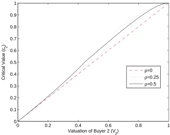
The solid line in Figure 1 shows the graph ofc(v2) for the cases withρ= 0,ρ = 0.25 and
ρ= 0.5. When ρ= 0, the graph ofc(v2) coincides with the 45◦ line. For positive correlation between V3 and V4 (ρ > 0), the graph of c(v2) is above the 45◦ line for all v2 ∈(0,1). As a result, there is a positive probability of inefficiency in the sense of selling the good to Buyer 2
in Auction 2 when Buyer 3 has a higher valuation than Buyer 2. The allocation is inefficient
in these cases.
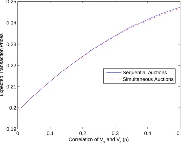
The expected transaction prices for sequential auctions are slightly higher than those for
simultaneous auctions. Figure 2 shows the transaction prices for these two types of auctions
0 0.2 0.4 0.6 0.8 1 0
0.1 0.2 0.3 0.4 0.5 0.6 0.7 0.8 0.9 1
Valuation of Buyer 2 (V
2)
Critical Value (c
2
)
ρ=0
ρ=0.25
[image:25.595.126.473.251.528.2]ρ=0.5
0 0.1 0.2 0.3 0.4 0.5 0.19
0.2 0.21 0.22 0.23 0.24 0.25
Correlation of V
3 and V4 (ρ)
Expected Transaction Prices
[image:26.595.116.484.245.537.2]Sequential Auctions Simultaneous Auctions
6
Conclusion
One important feature of Internet auctions which is ignored in the traditional auction
lit-erature is the entry of new buyers. In this paper, I show that, when multiple items of an
identical good are sold in sequential auctions and buyers have affiliated private valuation
over the good, entry would result in inefficient allocation of the goods. A less informed buyer
may win an auction even if her valuation is lower than other buyers. The inefficiency is a
consequence of information asymmetry between buyers. On the contrary, if all items are sold
in one multiple-object auction. The allocation is efficient, but sellers on average receive less
joint profit. The inefficiency remains possible if the mechanism is changed from a sequence
of ascending auctions to a sequence of sealed-bid second-price auctions.
This paper consider a simple situation to demonstrate the inefficiency due to entry to
sequential auctions. I conjecture the result to hold in a more general model, but rigid analysis
remains to be done in the future extension.
References
Ashenfelter, O. (1989). How auctions work for wine and art. Journal of Economic
Perspec-tives 3(3), 23–36.
Bajari, P. and A. Horta¸csu (2004). Economic insights from Internet auctions. Journal of
Economic Literature 42, 457–486.
Huang, C.-I., K.-P. Chen, J.-R. Chen, and C.-F. Chow (2008). Bidding strategies in parallel
internet auctions. Mimeo. National Taiwan University.
Milgrom, P. R. and R. J. Weber (2000). A thoery of auctions and competitive bidding,
II. In P. Klemperer (Ed.), The Economic Theory of Auctions, Volume 2. Edward Elgar
Publishing.
Ockenfels, A., D. Reiley, and A. Sadrieh (2006). Online auctions. NBER Working Papers
Wang, J. T. (2006). The eBay market as sequential price auctions – theory and experiments.
Mimeo. California Institute of Technology.
Weber, R. J. (1983). Multiple-object auctions. In R. Engelbrecht-Wiggans, M. Shubik, and
R. M. Stark (Eds.), Auctions, Bidding, and Contracting: Uses and Theory. New York
University Press.
Zeithammer, R. (2006). Sequential auctions with information about future goods. Mimeo.
University of Chicago.
Zeithammer, R. and C. Adams (2006). Modeling online auctions with proxy-bidding: