Solution of the boundary value problem for optimal escape in continuous stochastic systems and maps

Solution of the boundary value problem for optimal escape in continuous stochastic systems

and maps

S. Beri,1R. Mannella,2,1 D. G. Luchinsky,1A. N. Silchenko,1 and P. V. E. McClintock1 1_{Department of Physics, Lancaster University, Lancaster LA1 4YB, United Kingdom}

2_{Dipartimento di Fisica, Università di Pisa and INFM UdR Pisa, Largo Pontecorvo 3, 56127 Pisa, Italy}

共Received 15 March 2005; published 29 September 2005兲

Topologies of invariant manifolds and optimal trajectories are investigated in stochastic continuous systems and maps. A topological method is introduced that simplifies the solution of boundary value problems: The activation energy is calculated as a function of a set of parameters characterizing the initial conditions of the escape path. The method is applied explicitly to compute the optimal escape path and the activation energy for a variety of dynamical systems and maps.

DOI:10.1103/PhysRevE.72.036131 PACS number共s兲: 02.50.Ey, 05.40.Jc

I. INTRODUCTION

The understanding of activation processes in nonlinear stochastic maps and flows is one of the long-standing prob-lems of statistical physics. It attracts much attention in di-verse scientific contexts, e.g., in relation to stochastic reso-nance 关1兴, directed diffusion in stochastic ratchets 关2–4兴, nucleation in electrochemical systems 关5兴, the dynamics of VCSELs 关6–9兴 and gas lasers 关10,11兴, and the passage of ions through open ionic channels 关12兴 in biological mem-branes. From a mathematical point of view, the interest in activation problems derives in large part from the many stimulating topological discoveries that have been made in such systems关13–19兴.

The most promising steps toward a solution have been achieved in the regime of small noise intensities. In this asymptotic condition, the activation process can be described using anonequilibrium potential共or equivalently an activa-tion energy兲. The calculation of the activation energy re-quires the minimization of a “cost functional”S共x,t兲along a family of trajectories and the calculation of an optimal es-cape path that the system follows during the activation pro-cess with overwhelming probablity in the limit of zero noise intensity关5,20–24兴.

For a general system, the “potential”S共x,t兲is a multival-ued function of position x in the system state space 关4,5,15,20,25–34兴. Its calculation requires a topological analysis of the action surface关19,27,31,35兴and minimization over the set of all trajectories emanating from the initial steady state and terminating at x. The trajectory providing the escape from a basin of attraction with least cost is known as themost probable escape path共MPEP兲 关15,22,32兴. It is a heteroclinic trajectory lying on the intersection of the un-stable manifold of the initial state and the un-stable manifold of the boundary.

In general, the structure of the manifolds can be wildly singular and many heteroclinic trajectories may exist. The location of the MPEP is consequently a very difficult task: Many almost degenerate local minima appear in the action, and under these conditions the standard methods of minimi-zation do not provide a reliable means of extracting the glo-bal minimum. The multivaluedness of the potential at the

boundary makes minimization almost impossible to achieve in practice for escape from chaotic attractors关36兴, or in ac-tivation problems for systems where the basin boundaries are fractal 关37,38兴, or when the escape rate is enhanced by the presence of a chaotic saddle embedded in the basin关39兴.

In this paper we present a method of solving boundary value problems which significantly simplifies the investiga-tion in all of the difficult scenarios meninvestiga-tioned above. The same formalism applies both to maps and to continuous sys-tems. It is shown that all the results obtained for a map can be extended to continuous systems by taking the appropriate limit; quite counter-intuitively, however, not all of the results available for continuous systems can be exported to maps. We treat noise-activated escape in two-dimensional systems exhibiting unstable cycles, and in two-dimensional meta-stable and multimeta-stable maps.

In Sec. II we outline the Hamiltonian theory of large fluc-tuations in maps and introduce the MPEP, cost function, and the nonequilibrium potential or quasipotential. Section III is-cusses singularities in the quasipotential including caustics, cusp points, and switching lines, taking as an example the inverted van der Pol oscillator 共IVDP兲. A derivation of the boundary conditions is presented in Sec. IV. Section V pro-vides a linear analysis of the action surface and applies it to a simple 1D system, taken as an example. The parametriza-tion of the family of trajectories is discussed in Sec. VI. What we will refer to as theaction plotis introduced in Sec. VII. It represents an easy way to relate the topological prop-erties in the phase space to the features of the nonequilibrium potential. Its self-similar properties are discussed, and it is then applied in turn to a series of examples: The IVDP, the harmonically driven overdamped Duffing oscillator, and the Henon and Julia maps. In all cases the theory is tested by numerical simulations. Finally, Sec. VIII summarizes the re-sults and draws conclusions.

II. THEORY

xn+1=K共xn兲+␴␰n. 共1兲

Here兵xn其a set of coordinates describing the system,K共x兲is

a nonlinear function, and兵␰n其is a vector of stochastic

vari-ables mixed by the noise matrix␴. The stochastic variables

␰nare assumed to be Gaussianly distributed with

具␰n典= 0∀n 具␰n␰m典=⑀␦nm, 共2兲

where⑀is the noise intensity. In the rest of the paper, without loss of generality in the results the noise matrix␴is assumed to be the identity matrix.

A continuous system of the form x˙=K共x兲+␰共t兲 can be written as the limit for h→0 of the map xn+1=xn+hK共xn兲

+zn, where the new Gaussian variable zn=兰0

h_␰共

t兲dt has the momenta具z典= 0 and具z共t兲z共s兲典=⑀h␦共t−s兲. For this reason, in what follows, we will focus on the more general case of stochastic maps of the form共1兲and we will recover the re-sults for continuous systems using a limit procedure. The functionK共x兲 in Eq.共1兲is chosen such that the system dis-plays coexisting stable orbits.

When the noise intensity ⑀ is small, the system is ex-pected to spend most of its time in the vicinity of one of the stable states: Only occasionally will it move away from the stable state by a distance larger that

冑

⑀.

The probability of a transition from the initial pointxito a

final pointxfwith兩xf−xi兩⬎

冑

⑀can be expressed as

P共xf,xi兲=

冕

␥P关␥兴d兵␥其. 共3兲

Here the integration is taken along all possible paths␥ join-ing the initial and final states and the functional P关␥兴 ex-presses the probability of the system fluctuating along the path ␥. For a stochastic map of the form 共1兲, and a noise described by Eq. 共2兲, the probability P关␥兴 for a path ␥ =兵x₁¯xN其 can be written as

P关␥兴⬀exp

冋

−S关x1¯xN兴

⑀

册

. 共4兲

The functionS关x1¯xN兴 is acost functiondefined as

S关x1¯xN−1兴= 1 2

兺

n=0

N−1

␰n

2 _共5兲

with the constraint betweenxn and␰n expressed by Eq.共1兲.

In the asymptotic limit⑀→0, the transition probability共3兲 is dominated by the contribution from the path that mini-mizes the costS关␥兴. The contributions of other paths to the probability are exponentially suppressed. In other words, when ⑀→0, it is less and less likely that a transition will occur, but, on the other hand, when such an event manifests, it is exponentially likely to be according to the path that minimizes the cost.

The probability of the transition takes the asymptotic form

P共xN兩x0兲=zexp

冋

− Smin

⑀

册

, 共6兲

whereSmin is the least cost for the transition. The preexpo-nential factor共or prefactor兲gives a correction to the escape

probability related to the number of paths close to the path with least cost关40兴.

When the activation problem is considered explicitly, the initial state xi must be taken in the vicinity of one of the

stationary states, and the final statexfhas to be chosen on the

boundary of the basin of attraction of the stable structure. The path which realizes the escape with the least cost is known as themost probable escape path共MPEP兲. In order to solve the escape problem is necessary to work out the MPEP and calculate the cost along it. In this way, the probability of escape can be calculated using Eq.共6兲. The solution will be asymptotically correct in the limit⑀→0.

The cost functionSintroduced in Eq.共5兲has to be mini-mized with respect to the set of all possible noise bursts兵␰n其

and to the set of all possible intermediate coordinates兵xn其. It

is clear that Eq.共1兲gives a constraint between the values of 兵xn其 and 兵␰n其. The constraint is taken into account by

per-forming the minimization using the method of Lagrange un-determined multipliers. The auxiliary cost function

S ˜₌1

2

兺

n N

␰n

2

+␭n关xn+1−K共xn兲−␰n兴 共7兲

is introduced, where兵␭i其 is a set of Lagrangian multipliers.

The auxiliary functionS˜ must be minimized with respect to

␰i,xi,␭ias independent variables. The following relationships

are obtained from the minimization: xn+1=K共xn兲+␭n,

␭n+1=

冋

冏

⳵K

⳵xi

冏

x_n+1

册

−1

␭n. 共8兲

Equations共8兲 define an extended area-preserving map. The cost function can be considered as evolving along the trajec-tories according to

Sn+1=Sn+

1 2␭n

2

. 共9兲

The calculation of the transition probability can be now per-formed using Eq.共8兲to calculate the evolution of the system, combined with Eq.共9兲.

For a continuous system, the limith→0 gives

x˙=K共x兲+␭, 共10兲

␭˙_{= −}

冋

⳵K

⳵x

册

␭. 共11兲

Equations 共10兲 and 共11兲 can be seen as a set of equations describing an auxiliary Hamiltonian system. The Lagrange multiplier␭plays the role of a momentumpconjugate to the coordinate x. The Hamiltonian for this system is known as the Wentzell-Freidlin Hamiltonian

H共x,␭兲=1 2␭

2_{+␭K. 共12兲}

to the Lagrangian multipliers as momenta and we will use the notation␭ orp independently.

The equation for the evolution of the cost function along Eqs. 共10兲 and 共11兲 is Si+1=Si+

1

2h␭i2; in the limit h→0 it

reads as

S˙=1 2␭

2₌⳵H

⳵␭␭−H. 共13兲

Sevolves according to the equation for a classical action in the system described by the Hamiltonian 共12兲. Hamiltonian systems共10兲and共11兲, Hamiltonian共12兲, and Eq.共13兲for the cost function, can all be obtained in an alternative way through asymptotic analysis of the Fokker-Planck equation 关19,41兴.

Generally, there are infinitely many solutions of Eqs.共8兲 which emanates from the initial state x₀ and reach the final state xN; each of them having a corresponding cost. They

correspond to local minima of the cost function; however, in the limit of small noise intensity, the probability density for the system is dominated by the global minimum of the ac-tion, because the contributions of the other local minima be-come exponentially small. This property has been confirmed by analog experiments关42,43兴: The ensemble average of a large number of trajectories from an initial stationary point to a final one is found to be consistent with the least cost tra-jectory, and not with other local minima. In other words, only those trajectories corresponding to a global minimum can be observed in a physical experiment in the zero noise-intensity limit. For this reason, these trajectories are called physical and the ones corresponding to local minima un-physical关18兴.

The probability distribution is then defined by the mini-mum value of the costSmin共x兲= min兵Sm共x兲其, whereSmare the

costs calculated along different trajectories terminating inx. All the functionsSmare smooth, but the procedure of

mini-mization might produce nondifferentiability in Smin 关25,26,28兴. For nonequilibrium systems Smin is continuous, but it is not everywhere differentiable. The nondifferentiabil-ity of the cost function is a generic feature of nonequilibrium systems and has been intensively investigated 关1,18,25,26,28兴. Although not differentiable everywhere, nevertheless the functionSmincannot be arbitrarily irregular. First, S is nondecreasing along the trajectories of Eq. 共8兲. Second 关44兴, Smin is locally a Lipschitz function; i.e., for every pointx₀in the coordinate space, a neighborhood ofx₀ exists such that for any pair of pointsx1andx2

兩S_min共x₁兲−S_min共x₂兲兩⬍L兩x₁−x₂兩, 共14兲

whereLis a finite constant. The local Lipschitz condition is enough to imply differentiability almost everywhere关28兴.

It is known from the theory of nondifferentiable Lyapunov functions that, ifSmin is nondecreasing along the trajectories of Eq.共8兲and it is locally a Lipschitz function, then all theorems valid in the differentiable case can be gen-eralized关28兴. This allows the use ofS_minas anonequilibrium potential共orquasipotential兲for the system.

III. TOPOLOGY

The presence of singularities in the quasipotentialS_minis related to the presence of singular features in the pattern of solutions of Eq.共8兲or Eqs.共10兲and共11兲. They provide one of the main difficulties in the solution of the boundary values problem.

We consider the case of a continuous planar system pre-senting a saddle cycleSccoexisting with a stable equilibrium

point x0. The escape problem is formulated by setting the following boundary value conditions:

lim

t→−⬁

x=x0 lim

t→+⬁

x=Sc 共15兲

The picture for a two-dimensional map is similar.

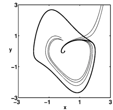
It is known from the theory of dynamical systems 关45兴 that the trajectories providing solutions of Eq.共11兲 emanat-ing fromx₀ fort→−⬁span a two-dimensionalLagrangian unstable manifold共UM兲in the four-dimensional phase space. The projections of these trajectories onto the coordinate space determine the pattern of escape trajectories. If we fol-low the motion of these trajectories, we expect three different behaviors, as summarized in Fig. 1, where the behavior of escape trajectories is shown for an inverted van der Pol 共IVDP兲system. It is an example of an autonomous system with a stable point coexisting with a saddle cycle described by the following equation:

[image:3.612.338.523.53.232.2]

mentumpជ to overcome the repelling force of the cycle and they are reflected back toward the initial stable state. A par-ticular trajectory separates the two families: It reaches the saddle cycle asymptotically 共for t→⬁兲 and tangentially 共p

→0 fort→0兲. In the extended phase space, such a trajectory lies on the intersection of the unstable manifold on the initial state and the stable manifold of the final cycle. The correct mathematical definition for a path having such a property is aheteroclinic trajectory.

It is classical result of the asymptotic theory of activation 关15–17,19,26,31兴that the most probable escape path must be a heteroclinic trajectory.

In a nonequilibrium system with saddles, the structure of both manifolds and patterns of trajectories can be singular 关13,15,17,19兴. The trajectories solution of Eq. 共11兲 may present multiple intersections in the coordinate space, and the pattern presents singular features such as caustics and cusp points. Caustics appear in the pattern as envelopes of trajectories; the cusps correspond to the merging of two separate branches of a caustic. A caustic can be generated by a family of trajectories during their motion toward the saddle 共where␭ is substantially different from zero兲or by trajecto-ries which are relaxing back toward the stable state共where␭ is near zero兲. Since the momentum of a trajectory becomes exponentially small as it approaches the saddle, the closer a trajectory gets to the limit cycle before being reflected, the more it resembles a purely relaxational trajectory during its motion toward the initial state and the contact with the caus-tics takes place far inside the cycle. For this reason, the in-ternal branch of the caustic always converges to the initial state.

In the region included by caustics, the escaping trajecto-ries intersect those trajectotrajecto-ries that are reflected back. Such apparent intersection results from projection onto the coordi-nate space, as the Cauchy theorem does not allow the trajec-tories to cross in the extended phase space and the “crossing” paths must have different values of momenta. In these re-gions, the Lagrangian manifold is threefold. What appears to be an intersection occurs between trajectories on different sheets of the manifold. A trajectory starts on one of the two external leaves of the fold. Then it eventually moves to the central leaf. In the projection, the leaf swap appears as a reflection by a caustic 关17,19兴. Once a trajectory is on the central leaf of the manifold, it stays there forever, because any further contact with the caustics is forbidden by the Cauchy theorem. Following contact with a caustic, the dy-namics of a trajectory continue on the central leaf of the manifold, and each of the trajectories on the central leaf may present the same behavior as the trajectories on the external leaves. In particular, heteroclinic trajectories other than the MPEP are present on the central leaf. Considering the pattern of trajectories on the central leaf of the manifold, it may present intersections similar to those observed for the full pattern. This means that the central sheet is folding again generating new caustics and cusps. This pictures repeats again and again in a self similar way.

In the region where different trajectories intersect, the ac-tion is multivalued. In the limit⑀→0, only the trajectories reaching a pointxwith least action can be observed experi-mentally. A continuous line separates the regions where the

physical trajectories are qualitatively different. Such a line is called theswitching line共SL兲 关17,19兴. Each point on the SL is reached by two different trajectories having exactly the same action. In the example of the IVDP, the SL separates the region where the physical trajectories have a momentum ␭ significantly different from zero from the regions where the physical trajectories are relaxing back toward the internal part of the cycle共having ␭⬃0兲. On the action surface, the switching line corresponds to the intersection共at a nonzero angle兲 of two sheets of the action surface. Cutting off the nonphysical parts of the action surface共i.e., those with non-minimum action兲, corresponding to the switching lines, we observe a nondifferentiability of the surface: The action is continuous on the SL, but the first derivative in the orthogo-nal direction switches abruptly between two different finite values.

IV. BOUNDARY CONDITIONS

In the previous sections, the complex, self-repeating, sin-gular structure of the manifold has been illustrated. All these are global properties, related to the nonlinear form ofK共x兲 and to the lack of detailed balance in the system. In order to set the boundary conditions properly, however, the shape of the manifold in the vicinity of the stationary states must be known.

In this section, we investigate the topology of the La-grangian manifolds in the vicinity of stationary points, for both maps and continuous systems, using linear analysis. We start from the simple case of a period-one stationary orbitxs

for a two-dimensional map. In the close vicinity of xs, the

extended map共8兲is rewritten as

␦xn+1=A␦xn+␭n,

共17兲 ␭n+1=A−1T␭n,

where␦xis the displacement from xsandA is the Jacobian

matrix of the original map calculated inxs. The point␦x= 0;

␭= 0 is a stationary point of map共17兲.

The unstable manifold ofxsis two dimensional and it is

spanned by the two unstable eigenvectors of Eq. 共17兲. As-sume first that the eigenvalues ␣1 and␣2 of A are real and satisfy兩␣1,2兩⬍1. The pointxsis a stable node for the original

map and a saddle point for the extended map共17兲. The ei-genvalues for the extended map are ␣1,␣2,␣1−1,␣2−1. The stable eigenvectors associated with the contracting eigenval-ues are calledes1 andes2 where the indexsindicates stable. The unstable eigenvectors are denoted byeu1andeu2. As the point is a stable focus for the original system, the two con-tracting eigenvectors have no␭ components and the stable manifold coincides with the coordinate plane. On the other hand, the expanding eigenvectors must have␭ components different than zero.

A generic pointx0=共␦x,␭兲 in the neighborhood of共xs, 0兲

x0=cs1␣1

n

es1+cs2␣2

n

es2+cu1␣1 −n

eu1+cu2␣2 −n

eu2. 共19兲 It is clear that the components ofxnalonges1,2shrink to zero and the components along eu1,2 expand. The eigenvectors eu1,2 span the unstable manifold. Once eu1,2 are known, an expression for the Lagrangian manifold can be obtained: The generic form for a point on the UM is obtained by setting cs1=cs2= 0 in Eq.共18兲. Separating the space and the␭ com-ponents we obtain

冉

xជ

␭ជ

冊

=cu1

冉

e ជu1x

eជu1␭

冊

+cu2

冉

e ជu2x

eជu2␭

冊

. 共20兲

Hereuជu1xandeu1␭represent the xand␭components of the eigenvectorseជu1,2. Writing the vectorsx and␭ explicitly in terms of their components x,y,␭x,␭y, a set of four linear

equations is obtained

冉

x y

冊

=

冉

eu1x eu2x

eu1y eu2y

冊冉

cu1 cu2

冊

冉

␭x

␭y

冊

=

冉

eu1␭x eu2␭x

eu1␭y eu2␭y

冊

冉

cu1 cu2

冊

.

Using standard linear algebra techniques, a linear relation amongxជand␭ជs may be obtained

冉

␭x

␭y

冊

=

冉

eu1␭x eu2␭x

eu1␭y eu2␭y

冊

冉

eu1x eu2x

eu1y eu2y

冊

−1

冉

x

y

冊

. 共21兲 The linear relation defining the UM is expressed in the form ␭ជ=Mxជ, with the matrixM defined as

M=

冉

eu1␭x eu2␭x

eu1␭_y eu2␭_y

冊

冉

eu1x eu2x

eu1y eu2y

冊

−1

. 共22兲

Consider now the case whenxsis an unstable focus. Here

the eigenvalues␣1,2are real and兩␣1,2兩⬎1. The point共xs, 0兲

is a saddle point of the extended map共17兲with eigenvalues

␣1,␣2,␣1 −1

,␣₂−1 and corresponding eigenvectorseu1,eu2,es1, andes2. The eigenvectors corresponding to expanding mo-tion have␭components equal to zero, while the components for contracting eigenvectors are nonzero. The unstable mani-fold coincides with the coordinate plane, while the stable manifold is expressed by the relation␭ជ=MxជwithM defined as

M=

冉

es1␭x es2␭x

es1␭y es2␭y

冊

冉

es1x es2x

es1y es2y

冊

−1

. 共23兲

We can summarize the effect of noise as follows. In the case of a stable point, noise introduces in the system two unstable directions and creates an unstable manifold in the extended phase space. For an unstable point, the situation is precisely the opposite: noise induces stable directions and creates the stable manifold. The situation differs, however, in the case wherexsis a saddle point of the noise-free system.

Here, one of the eigenvalues, e.g., ␣1 will have a modulus bigger than one, whereas for the other eigenvalue the

modu-lus is smaller. Stable and unstable directions are already present in the noise-free system. Noise then induces an ad-ditional stable direction and an adad-ditional unstable one. In the extended system, the unstable manifold is spanned by a “deterministic” eigenvectoreu1that has zero␭ components, and byeu2 having␭ components different than zero. In the same way, the stable manifold is spanned by a “determinis-tic” eigenvectores1and by a “fluctuational” eigenvectores2. The matrixM defining the unstable manifold of xsis given

by

M=

冉

0 eu2␭_x

0 eu2␭_y

冊

冉

eu1x eu2x

eu1y eu2y

冊

−1

共24兲

and in the same way the matrix defining the stable manifold is given by

M=

冉

0 es2␭x

0 es2␭y

冊

冉

es1x es2x

es1y es2y

冊

−1

. 共25兲

Consider now the case when the stationary point is a spi-ral node关46兴. Its eigenvalues␣1,2are complex conjugates. If 兩␣1,2兩⬍1,xsis a stable spiral node, a generic vector on the

unstable manifold is written as Eq. 共18兲 with coefficients cs1,2= 0, and the coefficientscu1,2are arbitrary complex num-bers. The matrix M defining the unstable manifold is then calculated in the same way as in the case of a stable focus. It should be noted that, although the coefficientseជu1,2are com-plex numbers, the final matrixMis real. The stable manifold forxsis defined by the simple relation␭ជ= 0.

In the case of an unstable spiral node, the stable and un-stable manifolds swap their roles: The unun-stable manifold is defined as␭ជ= 0 and the stable one by the matrixM.

Next, we investigate the case of a stable state of periodp. It is an orbit defined by兵xs1,xs2, . . . ,xsp−1,xsp其withxsp=xs1. A small neighborhood ofxsnis mapped by Eq.共8兲to a small

neighborhood ofxsn+1 and the shape of the manifold can be calculated in the close vicinity of each of the points of the periodic orbit. We start by describing the manifold close to xs1. In a small neighborhood ofxs1, the extended map can be written as

␦xn+1=

冋

冏

⳵K

⳵x

冏

x_s1

册

␦xn+␭n=A␦xn+␭n

␭n+1=

冋

冏

⳵K

⳵x

冏

x_s2

册

−1T

␭n=B−1T␭n, 共26兲

M=

冉

eu1␭x eu2␭x

eu1␭y eu2␭y

冊

冉

eu1x eu2x

eu1y eu2y

冊

−1

, 共27兲

with the same notation as in Eq.共23兲. The same calculation can be repeated in order to calculate the local shape of the unstable manifold in the neighborhood of the other points forming the periodic orbit. The casep= 2 will be considered explicitly below.

The case of a continuous flow, can be treated as usual as the limit forh→0 of the Euler integration scheme. Similarly a substitution of the Euler approximation f共xn兲=xn+hK共xn兲

into Eq.共17兲recovers a well-known result for the linearized Hamiltonian equations of continuous systems 共cf., e.g., 关17,31兴兲

再

␦x˙=K

⬘

共x0兲␦x+p,

p˙= −K

⬘

共x0_兲p, 共28兲 whereK

⬘

共x0_{兲 indicates the derivative of K共x兲 calculated at} x0_{. In matrix form Eqs.共28兲read as}

冉

␦x˙ p˙

冊

=

冉

B 1 0 −B

冊冉

␦x

p

冊

, 共29兲 whereB=K

⬘

共x0_{兲 and} ␦_{x is a small deviation of the} coordi-nate from the fixed point attractorx0_{. The generic point on} the unstable manifold is written in this case as x共t兲 =cu1eu1exp␣1t+cu2␷2

u

exp␣2t _{where c}

u1,2 are complex coeffi-cients and ␣1 and ␣2 are two positive eigenvalues corre-sponding to the unstable eigenvectors␷₁uand␷₂u. Accordingly, the connection between the momenta and coordinates on the unstable manifold of the linearized system can be written in a form similar to Eq.共21兲

冉

px

py

冊

=M

冉

x

y

冊

, 共30兲

where

M=

冉

eu1p_x eu2p_x

eu1p_y eu2p_y

冊

冉

eu1x eu2x

eu1y eu2y

冊

−1

. 共31兲

Equations共21兲and共30兲provide the choice of proper initial conditions for solution of the boundary values problem for flows and maps.

V. LINEAR ANALYSIS OF THE ACTION SURFACE

In the previous section, we addressed the problem of cal-culating the proper initial conditions to describe a trajectory performing the transition from a steady state to a remote final state. In order to calculate the transition probability, the non-equilibrium potential共or action兲must be also known. In this section we perform a similar analysis in order to describe the action surface in the vicinity of the stationary points.

Consideration of the relation␳⬀exp关−S/⑀兴shows that the quasipotential exhibits local minima corresponding to the stable equilibrium orbits of the original system. Similarly, it displays local maxima corresponding to unstable orbits. For this reason, we expect to be able to express the potential in a

neighborhood of stable equilibrium orbit as a quadratic form. For example, in the vicinity of a stationary point x₀, the potential can be approximated using a paraboloid

S关␦x兴=S0+ 1 2␦x

T

W␦x, 共32兲

whereS0is the potential exactly on the stationary point and

␦xrepresents a small deviation from x₀. The positively de-fined symmetrical matrix W describes the shape of the po-tential around the stationary point. The case of a stable peri-odic structure is similar: For a periperi-odic solution of periodp 兵xs1,xs2, . . . ,xsp−1,xsp其 with xsp+1=xs1, the potential is still quadratic, but its shape differs in the vicinity of the different points of the orbit.

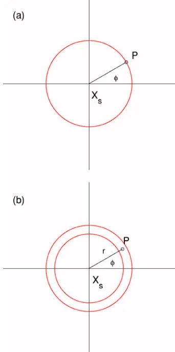
As shown in Fig. 2, a point in the vicinity of the stable orbit can be described by giving it an integer number indi-cating the closest point on the stable orbit, and a vector␦x giving the small displacement from that point. The potential can then be written as

S关i,␦x兴=S0+ 1 2␦x

T

Wi␦x, 共33兲

wherei is the integer defining the point on the stable orbit and Wi is the quadratic form defining the potential in the

vicinity ofxsi.

[image:6.612.342.522.54.340.2]

The case of a periodic orbit in the continuous system is a limit for the discrete system. The space in the vicinity of a FIG. 2. 共Color online兲 共a兲 Points in the vicinity of a period-3 orbit are described using the integeri苸关1_¯3兴and a real vector␦x

limit cycle can be described using a coordinate␥ along the cycle共in the same way as an integer was used in describing the space for a discrete system兲and a vector ␦x giving the small displacement from the cycle共as summarized in Fig. 2兲. The potential in this case is written as

S关␥,␦x兴=S0+ 1 2␦x

T

W共␥兲␦x, 共34兲

whereW共␥兲is the quadratic form describing the potential. It is clear from Eqs. 共32兲–共34兲 that a set of quadratic forms needs to be known in order to describe the boundary condition for the action. Similar to our calculation of the local shape of the Lagrangian manifold, we will start calcu-latingWfor the simplest case of a period-one orbit, and we will then move toward more complicated stationary struc-tures.

Consider the case of a period-1 stable point in a two-dimensional map. In the vicinity of the stable point xs, the

dynamics of the map can be linearized to obtain Eq.共17兲

␦xn+1=A␦xn+␭n,

共35兲 ␭n+1=A−1␭n.

From the previous section, we know that the relation ␭ =M␦x holds for the dynamics on the unstable manifold. Given a point␦xin the vicinity of the stable point, the cor-responding action has to be calculated along the trajectory emanating from the steady state atn→−⬁.

S=1 2

兺

_−⬁

1 ␭n

T_␭

n, 共36兲

where the T_{indicates the transpose operation on the matrix.}

Using the relation共21兲, the action can be rewritten as

S=1 2

兺

_−⬁

1

␦xn T

MTM␦xn. 共37兲

In order to express the action at the point␦x, it is necessary to express the coordinate␦xnas a function of␦x.

Manipulat-ing the first equation in Eqs.共17兲, the motion of the coordi-nate␦xon the unstable manifold is expressed by ␦xn+1=共A +M兲␦xn. In general we have␦x−n=共A+M兲−n␦x. Substituting

in the equation forS, the final expression for the action is

S=1 2

兺

1

⬁

␦xT共A+M兲−2nTMTM共A+M兲−2n␦x. 共38兲

The quadratic form W=共A+M兲−2nT_MT_M共A+M兲−2n _is

uniquely determined by the linearized system共17兲. Being a product of a matrix with its transpose, the eigenvalues ofW can be only positive or zero.

Consider now the case of a period-two stable orbit. In this case, the motion in the vicinity of the periodic orbit can be described using two different maps: one that maps points from a neighborhood ofxs1to a neighborhood ofxs2, and one that maps from a neighborhood ofxs2to a neighborhood of xs1.

␦xn+1=A1␦xn+␭n

␭n+1=A2−

T_␭ n

, ␦xn+1=A2␦xn+␭n ␭n+1=A1−

T_␭ n

, 共39兲

where A₁=兩⳵K/⳵x兩x_s1 and A2=兩⳵K/⳵x兩x_s2. The first map

de-scribes the transitions from the vicinity ofxs1 to the vicinity ofxs2, the second map does the opposite.

The potential is a sum of different contributions: The in-crease in the potential due to jumps from the vicinity ofxs1 to the vicinity ofxs2, and the contribution due to the opposite type of jump. The potential in a neighborhood ofxs1is writ-ten as

S=1 2

兺

_−⬁

0

␦x₀TM₁TA1共A2A1兲n共A2A1兲TnA1

T

M1␦x0

+1 2

兺

_−⬁

−1

␦x₀TM₁T共A₂A₁兲n_共A

2A1兲TnM1␦x0+S0. 共40兲

Here the first sum counts the contributions due to jumps fromxs2toxs1, and the second sum contains the contribution of the jumps fromxs1toxs2. This gives the following expres-sion for the quadratic form of the potential:

W1=M1

T

冋

兺

−⬁ 0

A1共A2A1兲n共A2A1兲TnA1

T

+

兺

−⬁ −1

共A2A1兲n共A2A1兲Tn

册

M1. 共41兲

The expression for the potential in the vicinity ofxs2 is ob-tained simply by exchanging the indices 1 and 2 in Eq.共41兲. The case of a generic period-p orbit is a simple generaliza-tion of Eq. 共41兲, where the contributions from p different types of jump have to be considered.

Now consider the case of a continuous system. The po-tential can be calculated in the vicinity of stationary struc-tures using either of two different approaches. The first con-sists of an application of the results obtained in the case of a map, using the limith→0 in the Euler discretization scheme. In the case of a stable point, this gives

S=S0+ 1 2␦x0

T

MT

冉

冕

−⬁

0

e−Ate−ATtdt

冊

M␦x0 共42兲

and

W=MT

冉

冕

−⬁

0

e−Ate−ATtdt

冊

M, 共43兲

and, for a limit cycle, it gives

W共␥兲=M共␥兲T

冉

冕

−⬁

0

e−Ate−ATtdt

冊

M共␥兲, 共44兲

where the parameter␥ is the coordinate along the cycle and

formalism guarantees the well-known relation between the potential and the momenta

pi=

⳵S

⳵xi

, 共45兲

which implies W=M. However, this result cannot be ex-ported straightforwardly to the case of discrete systems and, in the general case,W⫽M. An explicit example of this prop-erty will be given in the next section.

When an unstable state is considered, the situation can be different: The potential still exhibits a local maximum, but the simple quadratic description might not apply: The poten-tial might display singular features and be wildly nondiffer-entiable关17,21,31兴. Consider, for example, the IVDP system or the harmonically driven overdamped Duffing oscillator. In both systems a switching line converges asymptotically to the saddle cycle. As a result, a series of singularities in the action surface accumulate at the boundary and, given a small neighborhood of the cycle, the quasipotential there contains infinitely many nondifferentiable points.

A. Example: 1D system

To understand better the theory explained in the previous section, and in particular to show explicitly how the matrices M and W can differ for a generic map, we present as an example a simple one-dimensional linear system.

Consider the map xi+1=axi+␰i, where 兩a兩⬍1. The

sto-chastic process␰has zero mean具␰典= 0 and delta correlation 具␰i␰j典=⑀␦ij, where⑀is the noise intensity. The corresponding

extended map is

␦xi+1=axi+␭i,

共46兲 ␭i+1=

1 a␭i.

The eigenvalues of the extended system area and 1 /a. The stable manifold is defined by the relation ␭= 0 and the un-stable manifold by the relation␭= −共a− 1 /a兲x; these give the matrix共in this case a scalar, in actuality兲M= −共a− 1 /a兲. Mo-tion on the unstable manifold is regulated by the equaMo-tion xi+1=共1 /a兲xi. The potential of a given point xis calculated

using

S=1 2

兺

_−⬁

−1 ␭i

2 =1

2

兺

₁ ⬁

冉

a−1

a

冊

2

a2nx2 共47兲

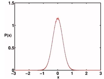
and the summation is performed in the standard way to ob-tainS=1₂共1 −a2_兲x2_{. Thus the matrixW is found explicitly as} W=共1 −a2_{兲. So the matricesW andM are different.}

In order to test these results, the system共46兲was solved numerically by Monte Carlo simulation. First the stationary distribution was obtained by consideration of a collection of 106 points共the system is obviously ergodic兲; the mean and the mean-square deviations were computed using the least-squares technique, and their values compared with the theory as shown in Fig. 3. The agreement was found to be excellent for a wide range ofa and⑀values.

As a second example, we consider a one-dimensional lin-ear continuous system x˙= −ax+␰. The parameter a is larger than zero and ␰ is a white uncorrelated Gaussian noise of intensity⑀. The extended Hamiltonian system is the limit as the integration steph→0 of the following map

␦xi+1=共1 −ah兲xi+h␭i,

共48兲 ␭i+1=

1 1 −ah␭i.

Repeating the same calculation as above, the eigenspaces for map 共48兲 are ␭= 0 and ␭= −1 /h关共1 −ah兲− 1 /共1 −ah兲兴x. We then have M= −1 /h关共1 −ah兲− 1 /共1 −ah兲兴. The action for a given point is calculated using the summation procedure

S=1 2h

兺

_−⬁

1 ␭n

2 =h

2

兺

₁ ⬁

1

h2

冋

共1 −ah兲− 1 1 −ah

册

2

共1 −ah兲2nx2.

共49兲 Performing the summation we get

S= 1

2h

冉

共1 −ah兲− 1 1 −ah

冊

2 _{共1 −ah兲}2 1 −共1 −ah兲2x

2_{, 共50兲}

which givesW= 1 /h(1 −共1 −ah兲2_{). For a given finite value of} h, the two matricesW andM are different. However, in the limith→0,M→2a, andW→2a. This recovers the standard result␭=⳵S/⳵xin the case of a continuous system.

VI. PARAMETRIZATION OF THE FAMILY OF TRAJECTORIES

The first step toward the solution of the escape problem is the identification of a proper way of parametrizing the family of escape trajectories. Since Eq.共21兲 holds, it is enough to provide a parametrization of the trajectories in the coordinate space.

[image:8.612.345.525.55.193.2]

choosing their initial conditions on a small circle共S1兲centred on the point共see Fig. 4兲.

For a two-dimensional map, a larger space of parameters is required: it is diffeomorph关47兴to a torusT1_=S1_⫻S1_{. The} initial conditions can be chosen on a small annulus with extreme radiir1andr2as shown in Fig. 4. We are interested in giving a parametrization for all possible trajectories in the pattern. It is clear that this requires particular care in the choice of the possible radiir₁ andr₂. A wrong choice ofr₁ andr2 might result in some trajectories in the pattern not to be sampled with this choice. In order to include all the tra-jectories in the pattern the radii r1 and r2 must be chosen such that the iterations of the annulus cover the full mani-fold. Providing the radii to be small enough, it is sufficient to satisfy the condition for the linearized system around the stationary point. Once the extreme radii are chosen, a pos-sible choice of parameters to describe the trajectories might be the radius r of a small circle about the origin and the angular position␾on it共see Fig. 4兲.

In the general case, the parameter space for a N-dimensional continuous system is diffeomorph to a 共N − 1兲-dimensional product of tori Tn_{; for a N-dimensional}

map; it is diffeomorph to aN-dimensional product of toriTn. Once initial conditions are defined on the coordinate space, the relation共21兲is used to work out the corresponding mo-menta.

VII. ACTION PLOT AND THE SOLUTION OF THE BOUNDARY VALUE PROBLEM

In this section we will show in a very effective way how the cost function can differ markedly for different escape trajectories and we will provide a tool for the solution of the boundary values problems.

To make it easier for the reader to follow the rationale of this section, we will stick to the case of a two-dimensional continuous system with a stable point and a saddle cycle; however, the discussion is actually more general and can be rewritten in an analogous way for the case of discrete sys-tems. The theory described in the previous sections allows us to give a parametrization of the trajectories emanating from an initial stable structure共for the noise-free case兲and span-ning the unstable Lagrangian manifold. Each of these trajec-tories emanates from the stable state att→−⬁and moves on the manifold in the 2n-dimensional phase space. In a projec-tion they appear to wander around on the coordinate space and eventually they may escape the basin of attraction of the initial stable state. In order to give a good representation of the escape energy, we consider each trajectory in the pattern. As this path is on the manifold, it can be unambiguously described, providing parameters in the way described in Sec. IV. The cost of the trajectory共namely, its action兲at the mo-ment of escape is thus expressed unambiguously as a func-tion defined on the parameter’s space. We will refer to the graphical presentation of the action as a function of the pa-rameters with the termaction plot.

The behavior of the trajectories during the fluctuation al-lows us to identify two different regions in the parameter space. Trajectories in the first region can cross the boundary of the basin of attraction and move further to reach the basins of attraction of different stable points. A second class of tra-jectories has a different kind of dynamics: They first move toward the basin boundary, but their momentum is insuffi-cient to allow them to cross the boundary; so they are re-flected back to the interior of the basin of attraction. The two regions are separated by closed curves in the parameter space corresponding to heteroclinic trajectories. The values of the action corresponding to the two different regions are signifi-cantly different. This may be explained in the following way: The cost functionS evolves along the Hamiltonian trajecto-ries according to Eq. 共13兲. Thus S˙ is a positively defined quadratic form in the auxiliary momentumpជ. Consider now the most probable escape path ␥0. During the fluctuation from the initial state toward the boundary, pជ is significantly different than zero and the cost function increases along the motion. As the system approaches the cycle,pជ decreases ex-ponentially and the optimal path converges to the limit cycle asymptotically. At the same time the cost function ap-FIG. 4. 共Color online兲 共a兲Possible way to parametrize the

[image:9.612.87.258.60.403.2]

proaches its asymptotic valueS0 corresponding to the acti-vation energy. Consider a path␥₁that is a perturbation of the optimal path. As a first possibility, the momentum兩pជ兩 on␥1 may be bigger than on␥0; as a result,␥1hits the cycle with a residual momentum. The cost function calculated along␥1 S₁=兰_␥

1兩pជ兩

2_{dt will be slightly higher than S}

0. Changing the trajectory continuously, it may have a cost S1 indefinitely close toS₀.

A second class of trajectories is also possible: Consider a trajectory ␥2 having a slightly smaller momentum than ␥0. Such a trajectory cannot overcome the repelling force of the limit cycle: It will come very close to the the cycle, but it will be repelled back toward the initial state. In this process, its costS2remains slightly smaller than the activation energy S0. During the motion toward the stable state, the momentum of␥2 stays very small and its cost will not increase signifi-cantly. After reaching some internal part of the basin of at-traction, the fluctuational motion will start once more and then the path will again move toward the limit cycle. During this second outward motion, its momentum becomes once more significantly different than zero. For this reason, when

␥2 away from the limit cycle, its cost will be significantly bigger than the activationS0. For this second class of trajec-tories, it is impossible to approach the cost S0 by changing the momentum continuously: A discontinuity in the cost function is always present. The different behaviors of the trajectories are summarized in Fig. 5.

According to the previous discussion, the cost function is a discontinuous function in the parameter space and the dis-continuities correspond to heteroclinic trajectories. The lowest-cost heteroclinic trajectory is the optimal path.

A. Self similarity of the action plot

The structure of the action plot for a generic nonequilib-rium system with a limit cycle can be very complicated. In Fig. 6共a兲the action plot is shown for the inverted van der Pol oscillator 共which will be discussed in more detail Sec. VII B兲. The features that will be described for this system are in fact very general, as will become apparent from the dis-cussion.

It is evident that the action plot has a wildly singular structure composed of broad, rounded, “hills”关for example, the region a–c in Fig. 6共a兲兴and very sharp “peaks.” At the edges of the hills, discontinuities are present, such as those marked by共1兲and共2兲in Fig. 6共a兲. According to the discus-sion above, each of the discontinuities corresponds to a het-eroclinic trajectory. The discontinuity with the lowest action 关marked as共1兲兴corresponds to the optimal path. On the other hand, the presence of other discontinuities suggests the pres-ence of other nonoptimal heteroclinic paths.

A zoom inside the first peak关Fig. 6共b兲兴reveals the pres-ence of closely similar structure: A smooth hill with two sharp peaks at each side. The discontinuities between hill and peaks are marked by arrows 共3兲 and共4兲. Inside the peaks, more hills and peaks are present. Two more discontinuities are marked with arrows共5兲and共6兲. Such a structure contin-ues indefinitely: Smaller and smaller hills exist, having higher and higher cost, and infinitely many discontinuities are present in the action plot.

[image:10.612.351.521.54.333.2]

The complex structure described here can be understood on the basis of the arguments introduced in Sec. VII. The first hills correspond to trajectories that cross the cycle dur-ing their fluctuation. The trajectories in the peaks have a significantly different cost: They are paths that have been reflected back and experienced the共cost-demanding兲 fluctua-tional motion twice. Inside the peaks, trajectories that are reflected back only once form the lower hills and trajectories FIG. 5. 共Color online兲Three different classes of trajectories are

possible for a system with a saddle cycle. ␥0 is the heteroclinic path: It reaches the cycle共dashed line兲asymptotically fort→+⬁;

[image:10.612.91.260.55.193.2]

␥1has a bigger momentum and crosses the cycle;␥2has insufficient momentum to reach the cycle and it is reflected back.

that are reflected back more than once form the internal peaks. This process goes on indefinitely and a hierarchy of trajectories can be built according to the number of reflec-tions back from the limit cycle that they experience.

The peculiar structure of the action plot can be used to locate the heteroclinic trajectories in the system and, in par-ticular, the optimal path. The optimal path corresponds to the minimum action heteroclinic path; other heteroclinic trajec-tories present in the system are nonoptimal.

B. IVDP system

As our first application, we study the activation energy for noise-induced escape in the inverted van der Pol oscillator 关48兴. The IVDP has already been mentioned above: It is a nonlinear oscillator containing terms describing losses and energy pumping. The dynamical model is

x¨= − 2␩共1 −x2兲x˙−x+

冑4

␩T␰共t兲, 共51兲 wherexis a dynamical variable and␰共t兲is a noise process. In what follows we will assume␰共t兲to be a zero-mean white Gaussian process. Its correlation function is 具␰共t兲␰共s兲典=␦共t −s兲. The intensity of the noise term is ⑀=

冑

4␩T whereT is the thermodynamic temperature of the system. The positive parameter ␩ in Eq. 共51兲 regulates not only the friction but also the pumping of energy into the system, which keeps the system away from thermodynamic equilibrium. As a result, the activation energy of this system displays a dependence on the value of␩that is nontrivial.

The dynamics of the system can be better understood with the substitutiony=x˙. In this way Eq.共51兲can be rewritten as

x˙=y,

y˙= − 2␩共1 −x2兲y−x+

冑4

␩T␰共t兲. 共52兲 In the coordinate space x-y, the noise-free dynamics of the system can be summarized as follows: The originO=共0 ; 0兲 is a stable equilibrium point. Its basin of attraction⍀is lim-ited by a saddle cycle. The stability of O depends on the parameter␩ and can be studied using linear analysis. In the vicinity ofO, the system becomes

冉

x˙ y˙

冊

=

冉

0 1

− 1 − 2␩

冊冉

x

y

冊

. 共53兲 The nature of the fixed point depends on the eigenvalues of the system␭1,2= −␩±

冑

␩2− 1. For values of␩smaller than 1, ␭1,2 are complex conjugates and the fixed point is a spiral node; for␩= 1 the system bifurcates,␭1,2become real andO becomes a stable node. The particular case␩= 0 correspond to an ideal harmonic oscillator of frequency 1.

When noise is added in the system, transitions from the stable origin to the limit cycle become possible. As discussed above, when the noise intensity is small, noise-induced es-cape from the basin of attraction of the fixed point is gov-erned by the properties of the most probable escape path, which is the heteroclinic trajectory of lowest cost. As the noise intensity ⑀ depends on both temperature and friction

coefficient, the parameter that becomes indefinitely small is Twhile the parameter ␩is held at a fixed value.

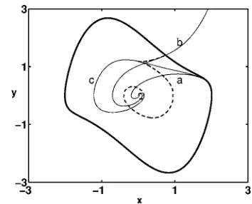
The action plot can be used successfully to calculate the activation energy in the system. As discussed in Sec. V, the pattern of trajectories is parametrized by setting the initial conditions on a small circle aroundO. The parameter space is thus diffeomorph to aS1_{. The action plot as a function of} the angular position ␾ on the circle is shown in Figs. 6共a兲 and 6共b兲. Interesting paths in the pattern of optimal trajecto-ries are shown in Fig. 7 together with singularities in the pattern共dashed lines兲.

The optimal escape path is marked with the letter “a.” It reaches the cycle tangentially fort→⬁. It corresponds to the discontinuity “a” in Fig. 6共a兲. Its action corresponds to the absolute minimum in the action plot. The path “b” in Fig. 7 corresponds to the top of the first hill in Fig. 6共a兲. Its cost is the maximum cost possible for a trajectory in the first hill. The path “c” in Fig. 7 is a nonoptimal heteroclinic path: It reaches the cycle asymptotically for t→⬁, but its cost is bigger than the activation energy 共the cost of path “a”兲. It corresponds to the discontinuity “c” in Fig. 6共a兲. It is pos-sible to move continuously from path “a” to path “c” along the first hill by continuously changing the parameter␾in the action plot.

Due to the central symmetry in the system of Eqs. 共52兲 two trajectories, such that one is the central reflection of the other, have the same cost. Due to this symmetry, the action plot, as a function of␾, has a period of␲and not 2␲. This means that two degenerate optimal paths are present in the system: the path “a” in Fig. 7 and that obtained from “a” by central reflection. In Fig. 7 the singularities in the pattern of optimal trajectories are shown as dashed lines. They are caustics, i.e., envelopes of Hamiltonian trajectories. It ap-pears clearly evident that acusp pointseparates the caustic into two branches: an external branch that hits the limit cycle, and an internal one that moves toward the origin. The trajectory “b” hits the limit cycle and simultaneously touches the caustic.

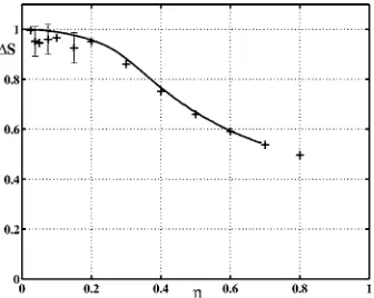
[image:11.612.345.522.54.197.2]

Carlo simulations共crosses兲in the limit of small noise inten-sity. Theoretical predictions and the results of the simulations agree well over a wide range of parameter values. The

small-␩asymptotic behavior of the activation energy corresponds to theoretical predictions based on adiabatic elimination of the fast rotation. The value␩= 0, corresponding to determin-istic motion of the system, may be reached only as a limit.

C. Harmonically driven overdamped Duffing oscillator

The inverted van der Pol oscillator described in Sec. VII B represents an archetypal nonequilibrium autonomous system with a limit cycle. In this section we show how the same method can be applied to the case of a nonautonomous system with limit cycles. In particular, we consider a poten-tial system kept out of equilibrium by a time dependent ex-ternal force. Consider a bistable potential U= −1₂x2+1₄x4 共Duffing potential兲and consider a particle moving according to

x˙= −ⵜU+Asin共␻t兲+

冑

⑀␰共t兲. 共54兲 Here the harmonic driving keeps the system away from equi-librium so that the detailed balance condition does not hold; the amplitudeAof the driving force is chosen large enough to be beyond the perturbative regime. The driving frequency is comparable with other time scales present in the system. The noise is introduced in the model by the stochastic vari-able␰. In what follows, we consider␰to be a standard zero-mean white Gaussian noise. Its correlation function is 具␰共t兲␰共s兲典=␦共t−s兲. The one-dimensional system 共54兲 is a nonautonomous; in order to make it an autonomous system, the following auxiliary system is introduced:

x˙1=␻,

共55兲 x˙₂= −ⵜU+Asin共x₁兲+

冑

⑀␰共t兲.

The system 共55兲 is two-dimensional, but it is now autono-mous.

The presence of the external driving transforms the equi-librium points to limit cycles of period 2␲/␻: The minima of

the potentialUforx= ± 1 become stable limit cycles and the maximum of the potential becomes a saddle cycle. The pres-ence of noise in the system might induce transitions from one stable cycle to the other one, across the unstable cycle. In order to calculate their probability, the extended system

x˙₁=␻, 共56兲

x˙2= −ⵜU+Asin共x1兲+p2,

p˙1= −Acos共x1兲p2,

p˙2= d2U

dx₂2p2,

has to be solved with a proper choice of boundary condi-tions:共x1;x2兲must be on the stable cycle fort→−⬁and on the saddle cycle fort→⬁.

The trajectories emanating from the stable cycle are a one-parameter family on the unstable manifold. A possible choice of parametrization can be as follows. Let the initial conditions be chosen to be of form 共x1;x2兲=(x1c共␾兲,x2c共␾兲

+␦), wherex1candx2care the coordinates of the stable cycle

at a given phase␾ and␦ is a small displacement in the x2 direction. The parameter␾parametrizes the family of trajec-tories. The optimal path found for the system is shown in Fig. 9. It is an heteroclinic trajectory reaching the saddle cycle fort→⬁.

D. Henon map

[image:12.612.353.524.54.191.2]

As a second example of the application of the formalism, we consider the case of a noise-driven Henon map. The Henon map, introduced in 1976 by Henon 关49兴, takes the form

FIG. 8. The activation energy for escape in the inverted van der Pol oscillator as a function of the␩parameter. The results of Monte Carlo simulations共crosses兲are compared with the action calculated using the action plot technique共full curve兲. Error bars are shown for some of the points.

[image:12.612.91.259.56.190.2]

再

xn+1=a−xn

2

+byn+␰n

yn+1=xn.

冎

共57兲

Herexn andyn are the dynamical variables;aandbare real

parameters for the system and兵␰n其 is a set of uncorrelated

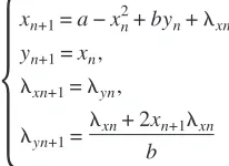
white Gaussian noises of intensity ⑀. Different regimes of complexity can be obtained in this system by tuning the pa-rameters in an appropriate way共see, for instance,关49,50兴兲. In this section we will apply the technique described to regimes which are more and more complex. We start with a choice of parameters 共a= 1.1, b= −0.3兲 corresponding to one stable period-1 orbit and one attractor at infinity. The boundary of the basin of attraction is then smooth 共nonfractal兲 and a period-1 saddle orbit is present in the boundary. The ex-tended system corresponding to Eq.共57兲is

冦

xn+1=a−xn2+byn+␭xn,

yn+1=xn,

␭xn+1=␭yn,

␭yn+1=

␭xn+ 2xn+1␭xn

b

冧

共58兲

and the activation energy evolves along the trajectory ac-cording toEn+1=En+

1 2␭xn

2_.

In the extended system共58兲, the stable orbit becomes a saddle, and the escape trajectories span its unstable manifold. According to the general theory, it is a two-dimensional sur-face and the trajectories form a two-parameter family. From the linearization of the system 共58兲, the manifold can be defined in a neighborhood of the initial state and a linear relation共21兲 between coordinates and momenta is obtained. The matrix Mij, which appears in Eq. 共21兲, is here a 2⫻2

matrix.

A suitable choice for the parametrization of the manifold about the initial state is the radius and the angular position on a small circle around the point. The action plot is here a functionS1_⫻S1_{→R. The situation is very complicated, but a} global minimization is still possible and an “energy minimal” escape trajectory can be found, as shown in Fig. 10. The theoretical path obtained using the actionplot techniques is shown as a dashed line. It is compared with the results of a Monte Carlo simulation using a noise intensityD= 0.02. The two paths are in almost perfect agreement. The optimal tra-jectory leaves the initial state along its unstable manifold, reaches the boundary, and then drifts in an almost noise-free way toward the saddle at共−1.88; −1.88兲. The escape takes place at the saddle point.

In order to show that the method described is general, we tune the parameters to a particularly interesting regime where the basin boundaries are fractal. Considering a= 1.405 and b= −0.3, the system displays a stable period-2 orbit共xs1;xs2兲 coexisting with a stable attractor at infinity. The boundary of the basin of attraction is fractal and a period-3 accessible orbit 关37,51兴 is embedded in it. It is an example of locally disconnectedfractal boundary共see the discussion in关52兴for the classification of fractal boundaries兲. The correct math-ematical definition of this property is the following:

Definition 1 (locally disconnected set). A setA is defined

as locally disconnected if, given a point x in the set, there exists a small ball of radius⑀, such that for every␦ a point y苸A exists for which兩x−y兩艋␦ and no connected subset of Acontaining bothxandyand lying wholly in the⑀-ball can be found.

The extended system共58兲must be solved with the correct initial conditions in a small neighborhood of the period-two stable orbit. The trajectories solution of Eq.共58兲span a two-parameter family on the two-dimensional unstable manifold. In order to provide appropriate initial conditions, the full extended system 共58兲is linearized in the vicinity of one of the points in the stable orbit, for instancexs1. The expanding subspace was calculated using linear analysis, and the matrix relating coordinates and momenta on the manifold were worked out.

[image:13.612.344.522.55.197.2]

Although the action plot for the system is again very com-plicated, global minimization can be performed to obtain the MPEP. The results of the theory agree very well with the numerical output of Monte Carlo simulation as shown in Figs. 11 and 12. The escape trajectory leaves the period-two stable cycle along the optimal path and reaches the boundary through the stable manifold of the accessible period-three orbit. Investigation of the almost noise-free dynamics along the fractal boundary lies beyond the scope of the present work but has been discussed in general terms elsewhere关37兴. In this section, we have demonstrated the method explic-itly for the Henon map, first for a parameter choice corre-sponding to a stable period-one orbit and smooth basin boundaries and, second, for the more complex case of a period-two stable orbit and fractal basin boundaries. It is clear that the method can be applied in the general case of a period-n initial orbit: The two-parameter characterization of trajectories still holds, and the procedure described above also applies to the case of a period-n initial state.

E. Julia map

[image:13.612.115.218.239.314.2]

boundaries arelocally connected共LC兲 关52兴. The mathemati-cal definition of a lomathemati-cally connected basin boundary is as follows:

Definition 2 (locally connected set). A set A is defined connected if, given a point xin the set and a small ball of radius ⑀, around it, a ␦ such that for every y苸A with 兩x −y兩艋␦ there is a connected subset of A containing both x andyand lying wholly in the⑀-ball.

An example of this kind of fractal boundary is given by the following analytic map关52,51兴

xn+1=xn

2 −yn

2

+axn+␰xn,

共59兲 yn+1= 2xnyn+axn+byn+␰yn.

Herexn andynare two dynamical variables andaandbare

real parameters. The two stochastic terms ␰xn and ␰yn are

Gaussian and ␦ correlated with intensity ⑀. Choosing the

parameter a= 0.7 and b= 0.5 共a choice made according to 关50兴兲, the system has a stable fixed point at 共x,y兲=共0 , 0兲 whose basin boundaries are fractal and locally connected. In particular, the basin boundaries are a Julia set关53兴, histori-cally an example of fractals that were investigated by the French mathematician Gaston Julia共1893–1978兲.

The presence of the two noise sources␰xnand␰ynmakes it

possible to observe transitions from the stable point of Eq. 共59兲to the basin boundary. Previous investigation of the ac-tivation process in this system was reported by Grassberger. His analysis was difficult due to the fractal structure of the boundaries; in particular, he failed to locate the correct boundary conditions.

Using the asymptotic approach in the limit of ⑀→0, the extended map is obtained

xn+1=xn

2 −yn

2

+axn+␭xn, 共60兲

yn+1= 2xnyn+axn+byn+␭yn,

␭xn+1=

共2xn+1+b兲␭xn

J −

共2yn+1+a兲␭yn

J ,

␭yn+1=

2yn+1␭xn

J +

共2xn+1+a兲␭yn

J .

The trajectories solution of Eq.共60兲forms a two-parameter set in the extended four-dimensional space. The space of parameters is once more diffeomorph to a torusT2. The tra-jectory that minimizes the cost is shown together with the results of numerical simulations in Fig. 13. The optimal es-cape path agrees with the results of the numerical simula-tions. It reaches the boundary asymptotically and the escape takes place following a saddle cycle of period 9.

[image:14.612.352.520.55.194.2]

In order to compare more accurately the theoretical MPEP with the results of numerical simulations, time series of thex variable for both the theoretical MPEP and the numerical one are shown together in Fig. 14. Excellent agreement is evi-dent. The theoretical MPEP escapes through the period 9 orbit. but the numerical MPEP escapes earlier due to finite FIG. 11. 共Color online兲 Comparison of theory and experiment

for the escape problem in the Henon map 共parameters are a

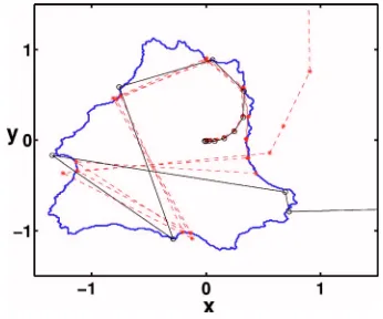
[image:14.612.89.260.57.201.2]

= 1.405 andb= −0.3兲. The solid line is a numerical realization of the escape; the dashed line is the theoretical trajectory found using the actionplot. Agreement between them inside the domain of attraction is excellent. On the boundary, the numerical dynamics diverges from theory due to the finiteness of the noise.

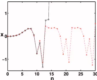
FIG. 12. 共Color online兲The theoretical MPEP共dashed line兲for the Henon map compared with an escape path共solid line兲found by numerical simulation in the iteration-coordinate domain: n repre-sents the number of iterations共the originn= 0 is chosen arbitrarily兲 andxis the coordinate. The parameters area= 1.405 andb= −0.3. Agreement between experiment and theory is excellent.

[image:14.612.89.260.519.660.2]