Modelling and controlling of stochastic dynamics of complex
nonlinear systems
Dmitry G. Luchinsky
a, Peter V.E. McClintock
a, Alexandr N. Silchenko
a, Vadim N.
Smelyanskiy
b, Mark I. Dykman
c.
a
Department of Physics, Lancaster University, Lancaster LA1 4YB, UK;
bNASA Ames Research Center, Mail Stop 269-2, Moffett Field, CA 94035, USA;
cDepartment of Physics and Astronomy, Michigan State University, East Lansing, MI 48824.
ABSTRACT
An application of the path-integral approach to an analysis of the fluctuations in complex dynamical systems is discussed. It is shown that essentially the same ideas underly recent progress in the solutions of a number of long-standing problems in complex dynamics. In particular, we consider the problems of prediction, control and inference of chaotic dynamics perturbed by noise in the framework of path-integral approach.
Keywords: Fluctuational transitions, chaos, control of chaos, nonlinear dynamical inference
1. INTRODUCTION
Almost all systems, whether in nature or in technology, are noisy and nonlinear and, in general, their behaviour canonlybe understood if the nonlinearity and noise are taken explicitly into account. Such studies are of wide applicability to many branches of science and technology, where identical model equations often arise in diverse contexts.
One of the ultimate goals of such studies is prediction and control of complex stochastic dynamics – the prob-lem that was challenging researchers for decades. A particular challenging aspect of this probprob-lem is an analysis of fluctuations in systems with complex geometrical structure of an attractor or/and attractor’s boundaries, such as chaotic systems.
A traditional approach to the problem of prediction in the context of stochastic nonlinear dynamic would be to calculate the probability of various events in such systems, including e.g. the probability of fluctuation-induced transitions between coexisting states.1 As a result the dynamical information is usually lost and traditional approach does not allow the development of methods of dynamical control. Moreover, in the actual experimental situation the model is not usually known exactly from “first principles” and one is faced with the problem of inferencing a parametric model from the measured time-series data.
Therefore, a few fundamental distinct problems can be formulated in the context of research of complex dynamical systems:
• inference of the parametric dynamical model from the experimental time-series data;
• calculations of the probability distribution function;
• development of the methods of dynamical control.
These problems are usually considered in the context of distinct scientific disciplines, see e.g..2–4
We will show, however, that the problems of prediction, control, and inference of complex dynamical systems can be addressed in a general framework of the path-integral approach to the analysis of the fluctuational trajectories.5, 6 The unifying theme of this approach is the idea that the solution of all above mentioned problems
Further author information: (Send correspondence to D.G.L)
D.G.L.: E-mail: [email protected], Telephone: +44 1524 593079
in the limit of weak to moderate noise-intensities requires global minimization of similar probability density functionals. An additional important advantage of this approach is that it allows to use similar calculations for both maps and flows. A special care should be taken, however, in transformation from stochastic to dynamical variables in each case.
The paper is organized as follows. In the Sec. 2 we introduce the probability density functional to have a given fluctuational trajectory in dynamical flows and maps. In the Sec. 3 we apply the path-integral approach to the analysis of the noise-induced escape from a chaotic attractor via fractal basin boundary. In the Sec. 4 we demonstrate that the same approach can be used to solve the problem of energy-optimal control of migration in chaotic attractor. Finally, in Sec. 5 we apply path-integral formulation to the solution of infer parameters of chaotic system from the experimental time-series data.
2. PROBABILITY DENSITY FUNCTIONAL OF FLUCTUATIONAL
TRAJECTORIES
Consider a dissipative stochastic dynamical system described byL-dimensional map
xn+1=f(xn) +σξn, ξαnξβn=δnnδαβ, (1)
wherexn, ξn∈RL, andσis a matrix that mixes white Gaussian noisesξn. Note that particular casef(xn) =xn+
hK(xn) corresponds to a prepoint Euler discretization scheme for Langevin systems of equations corresponding
to dissipative dynamical flow
˙
x=K(x) +σξ(t), (2)
ξα= 0, ξα(t)ξβ(s)=δ(t−s)δαβ,
where xn = x(tn), tn =nh, h = (tf−t0)/N with the initial and final times t0 and tf. In both casesx is a
L-dimensional vector of dynamical variables describing the systems (1) and (2). K(x) is a non-linear vector field (which may depend explicitly on time),ξ(t) is a zero-mean Gaussian noise.
The form of the probability functional is determined by the properties of the dynamical noise ξ(t).6, 7 It is clear from the eq. (1) that the probability ρ(xN, tf|x0, t0) of fluctuational path {xn} connecting attractor
SAwith arbitrary pointSB in its basin of attraction is deterministically related to the probabilityρ[ξn] for the random force to have corresponding random realization{ξn}. Taking into account that for white Gaussian noise
ξn at each time step are independent on each other the later probability is given by (cf.1, 8–11)
ρ[ξn] N−1
n=0
dξn= N
n=0 L
l=0
dξn √
2πexp
−1
2ξ
T n,lξn,l
. (3)
Changing to dynamical variables we have the probability for the system (1) to have fluctuational trajectory{xn}
in the form
ρ[xn] N−1
n=0
dxn= 1
(2π)NLdet (D)
N−1
n=0
dxnexp
−1
2(xn+1−f(xn))
TD−1(x
n+1−f(xn))
, (4)
where D = σσT. In the transformation from (3) to (4) we have neglected the Jacobian of transformation
J(xn) =∂∂(x(ξnn+11,ξ,1n...x2,...ξn+1nL,L)). This Jacobian is 1 for the maps. However, for the flows it is essential different from 1
as follows from the mid-point finite difference approximation of (2)xn+1=xn+hK(xn∗) +σznwhereσ =σ√h
and x∗n = (xn+xn+1)/2. It can be easily seen that in this case to the first order approximation in h the
Jacobian of transformation isJ(x)≈1−h2Ll=0∂K∂xl(xn) n,l (cf.
12–14). This term turns out to be unimportant in
of the inference one does not assume necessarily the presence of large deviations and the prefactor term gives the dominant contribution to the reconstruction of the system dynamics from the time-series data.
Finally the probability density functional F[x] over the trajectory xn of system (1) and of system (2) (in
Euler approximation) is given by the following equation
F[x] = J(x)
(2πh)NLdet (D)exp
−1
2h
N−1
n=1
(xn+1−f(xn))TD−1(xn+1−f(xn))
, (5)
whereJ(x) = 1 andh= 1 for the maps (1) andJ(x)≈1−h2Ll=0∂Kl(xn)
∂xn,l andhis the time step of discretization for the flows (2).
2.1. Extremal fluctuational paths
Suppose we are interested in calculation of the probability to find a dynamical system at any point in the basin of attraction Ω of some attractorA. If the distance from the attractor is much larger then the square root of largest eigenvalue ofD we can assume that the noise is small and in this sense to analyze the probability of large deviations fromA.
As we have mentioned above in the analysis of large deviations the prefactor can be neglected and we can proceed to obtain equations for the most probable fluctuational paths via analysis of the global minimum of the energy functional for the system (1)
S= 1 2
N
n=1
ξnTξn, under condition xn+1−f(xn)−σξn = 0, (6)
on a discrete timen= 0, ..., N, wherex0 belongs to the attractor andxN is an arbitrary point in the basin of
its attraction. In a particular case of the escape from the basin of attractionxN belongs to the basin boundary.
The corresponding results for the flows can be obtained as a limiting case off(xn) =xn+hK(xn) withh→0.
Introducing Lagrangian multipliersλn we have to minimize11 effective functional
S∗= 1 2
N
n=1
ξnTξn+ N
n=1
λTn(xn+1−f(xn)−σξn), (7)
with respect to independent variations ofξn,λn, andxn leading to 2L-dimensional map of the form11
xn+1=f(xn) +σσTλn,
λn+1={f(xn+1)}−1λn. (8)
To obtain corresponding results for the flows we substitute Euler approximationf(xn) =xn+hK(xn) into (8).
Taking into account thatσgoes intoσ=σ√hwe obtain
˙
x=K(x) +Dp,
˙
p=−K(x)p, (9)
which are well-known15, 16 Hamilton’s equations for the flows in the extended phase space. Here we introduced the notations for vanishingly smallh: λn→p(t),xn→x(t), (λn+1−λn)/h→p˙, and (xn+1−xn)/h→x˙.
This clarifies physical meaning of the Lagrangian multipliers in (8) as quantities equivalent to momenta in continuous equations and show the connection between eqs. (8) the Hamilton’s equations for the flows.
2.2. Boundary conditions
To describe initial conditions we assume for simplicity that the attractor has a fixed pointx0 of period one and linearize eqs. (8) about this point to obtain
δxn+1=f(x0)δxn+Dλn,
λn+1=f(x0)−1λn. or in matrix form
δxn+1
λn+1
=
A D
0 A−1
δxn
λn
(10)
whereA =f(x0). The unstable manifold of x0 is a two-dimensional hyperplane spanned by the two unstable eigenvectors vu1 and v2u of (10). The generic point on the unstable manifold is written as vn+1 = α1v1uµn1 +
α2v2uµn2 where α1,2 are complex coefficients and µ1 and µ2 are two multipliers corresponding to the unstable
eigendirections. Separating theδxand the λcomponents we obtain linear relationship between xand λfor a 2-dimensional map in the form
λx λy =M x y
, where M =
v1λx v2λx
v1λy v2λy
v1x v2x
v1y v2y
−1
. (11)
Similarly a substitution of Euler approximationf(xn) =xn+hK(xn) into (10) recovers a well-known result for
the linearized Hamiltonian equations for continuous systems (cf. e.g.6, 17, 18)
δx˙ =K(x0)δx+Dp,
˙
p=−K(x0)p. or in matrix form
δx˙ ˙ p = B D
0 −B
δx p
(12)
whereB =K(x0) andδx is small deviation of the coordinate from the fixed point attractor x0. The generic point on the unstable manifold is written in this case asv(t) =α1v1uexpλ1t+α2vu2expλ1twhereα1,2are complex coefficients and λ1 and λ2 are two positive eigenvalues corresponding to the unstable eigenvectors v1u and v2u.
Accordingly the connection between the momenta and coordinates on the unstable manifold of the linearized system can be written in the form similar to (11)
px py =M x y
, where M=
v1px v2px
v1py v2py
v1x v2x
v1y v2y
−1
. (13)
Equations (11) and (13) provides the choice of a proper initial conditions for the solution of the boundary value problem for flows and maps. For the two-dimensional flows and three-dimensional maps considered in the following chapters the corresponding unstable manifolds can be parameterized using two-parameter sets.
In particular, the activation processes in the systems (1) and (2) in the limit of small noise intensity is gov-erned by the most probable escape path that drives the system from the point attractorx0at t0→ −∞to the
saddle orbit SB at tf →+∞.
The analysis of the stable manifold of an unstable (or saddle) structure is performed in a similar way.
2.3. Experimental investigation of the large deviations
One of the important points to bare in mind is that the optimal fluctuational paths can be measured directly in the experiment as was suggested by Dykman et al.19 In this technique the dynamics of the system is followed continuously. Several dynamical variables of the system and the random force (when available20) are recorded simultaneously, and then the statistics of all actual trajectories along which the system moves in a particular subspace of the coordinate space is analysed. The theory predicts and the experiment demonstrates19–25 that so-calledprehistory probability distributionof such trajectories moving the system from the equilibrium state to the remote state are sharply peaked about the optimal fluctuational path.
force, it will occasionally fluctuate to a given point in the attractor basin. In doing so in the limit where the noise intensity tends to zero, the system will follow very closely the “deterministic” optimal fluctuational trajectories.
This technique has been mainly developed through the applications to the analysis of fluctuations in electronic circuits23and only recently it was extended to the investigations of the fluctuations in real physical systems. In particular, in the work by Hales and co-authors25the prehistory distribution was observed experimentally using a semiconductor laser with optical feedback.
We emphasize that the possibility of experimental investigation of the probability density functional of large deviations is an additional important advantage of the path-integral approach to the analysis of the fluctuations in complex stochastic nonlinear systems, where neither stationary probability distribution nor the PDF (5) are known theoretically. As we will show in the next two sections such experimental measurements can be very helpful in the analysis of escape and control problems in chaotic systems in particular.
3. ESCAPE THROUGH A FRACTAL BOUNDARY
The mechanism of fluctuational escape from a chaotic attractor (CA) through a fractal basin boundary (FBB) represents one of the most challenging unsolved problems in fluctuation theory.1, 8, 11, 26 The unpredictable and highly complex stochastic behavior of such systems arises in part from the presence of limit sets of complex geometrical structure, and in part from the fractality of the basin boundary.27, 28 For this reason, the central question – whether or not there exists a generic mechanism for fluctuational transitions through the FBB – has remained unanswered.
In this Section we show that a generic mechanism of fluctuational transition between co-existing CAs separated by an FBB can be found using experimental analysis of the probability distribution of the fluctuational trajec-tories described above. Such an analysis reveals a unique solution for the escape problem and the corresponding boundary conditions both on the attractor and attractor boundaries and facilitates further investigations of the noise-induced transitions in chaotic systems based on the path-integral approach.
To demonstrate the existence of this escape mechanism, we take as an example the two-dimensional map introduced by Holmes.29 The properties of this map, including the structures both of its CA and of its locally disconnected FBB, are generic for a wide class of maps and flow systems.30 This fact, taken with the results of our investigations of escape in other systems, allows us to conclude that the escape mechanism we describe is indeed a typical one. The Holmes map is
xn+1 = yn (14)
yn+1 = −b xn+d yn−yn3+ξn,
whereξn is zero-mean, white, Gaussian noise of varianceD. Due to symmetry, the noise-free system (14) with
b= 0.2 and 2.0≤d≤2.745 has pairs of co-existing attractors, the basins of which are separated by a boundary that may be either smooth or fractal, depending on the choice of parameter values. We choose for our studies
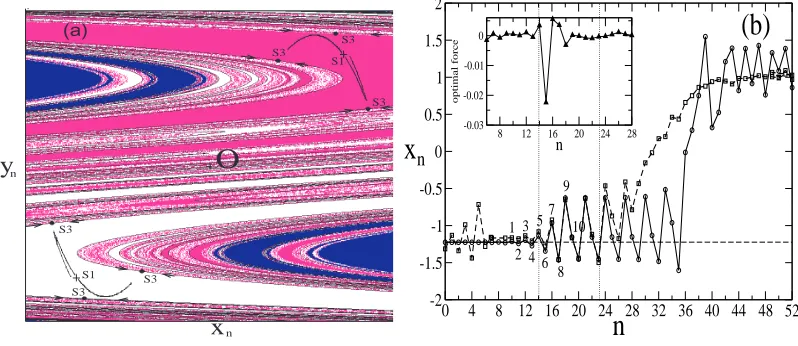
b = 0.2 andd = 2.7, which corresponds to there being two co-existing CAs separated by a locally disconnected FBB (see Fig. 1). The fractal dimension of the boundary has been determined numerically (dim = 1.84472) by using the “uncertainty exponent” technique introduced in.31 The chaotic attractors in (14) appear as the result of a period-doubling cascade and, for the parameters chosen, each of them consists of two disconnected parts.
We have modelled the system (14) numerically, exciting it with weak noise, and have collected trajectories that include escape paths from one CA to the other, and also the corresponding realisations of noise that induced these transitions. By ensemble averaging a few hundred such escape trajectories and noise realisations, we have obtained the optimal escape path and the corresponding optimal force, which are shown in Fig. 1(b). The results of this statistical analysis allow us both to determine the boundary conditions near the CA and the FBB, and to demonstrate the uniqueness of the MPEP. It can be seen in particular that, in leaving the CA, the system (14) falls into a small neighbourhood of the saddle point of period 1 (S1) located between its two disconnected parts and having the multipliersρ1= 0.118975 andρ2= 1.681025. Its stable manifolds separate the parts of the
S1 S3
S3 S3
S3 S3
S3
S1
x
y
nn
O
(a)0 4 8 12 16 20 24 28 32 36 40 44 48 52
n
-2 -1.5 -1 -0.5 0 0.5 1 1.5 2
x
8 12 16n 20 24 28-0.03 -0.02 -0.01 0
optimal force
n
(b)
8 7
6 5
4 3
2 1
9
[image:6.595.106.505.74.247.2]10
Figure 1.(a) The co-existing chaotic attractors (filled black regions) and their basins of attraction represented by grey and white respectively. The accessible boundary saddle points of period 3 are shown by the small filled black circles labelled S3. Their stable manifolds are shown as full black lines. The saddle points of period 1 are shown by the crosses labelled S1. The saddle point at the origin is labelled O. (b) The most probable escape path (dashed line) connecting the CA with the period-3 saddle cycle lying on the fractal boundary, obtained from the Monte-Carlo simulations withD = 10−5. The optimal path found by the solution of the boundary-value problem is shown as a solid line. Thex-coordinate of the saddle point S1 is shown by the horizontal dashed line.
(S3) with multipliersρ1= 0.001016 andρ2= 7.875512. Calculations have shown that, for the chosen parameter values, S3 lies within the FBB. Moreover, its stable manifold (solid black line in Fig. 1(a)) is dense in the FBB and detaches the open neighborhood, including an attractor, from the FBB itself. This allows us to classify it as an accessible boundary point.32
An analysis of the structure of escape paths inside the FBB has shown that the homoclinic saddle points play a key role in its formation. In the system (14), we observe an infinite sequence of saddle-node bifurcations of period 3,4,5,6,7..., which occur at parameter valuesd3< d4< d5< d6< d7... and are caused by tangencies of the stable and unstable manifolds of the saddle point O at the origin. The homoclinic orbits appearing as a result of these bifurcations were classified earlier as original saddles, and it was also shown that their stable and unstable manifolds cross each other in a hierarchical sequence.32 To characterize this hierarchical relation between original saddles, it is reasonable to introduce a parameterµequal to the ratio| ln(ρ1(P)) |/ln(ρ2(P)),
whereρ1 andρ2 are the multipliers of a saddle pointP. Calculations have shown that, for the original saddles
of period 3,4,5,6,7,8... in (14), the following hierarchical sequence of indexµ values occurs: µ3 = 3.339, µ4 =
3.08, µ5 = 2.999, µ6 = 2.339, µ7 = 1.958, µ8 = 1.539. Moreover, the values of index µ corresponding to the
other homoclinic saddle cycles are close to zero. Correspondingly the probability of finding the system in their neighbourhood tends to zero.
These results allows us to infer features of a fluctuational transition through a locally disconnected FBB that are probably generic, as follows: (i) it always occurs through a unique accessible boundary point; and (ii) the original saddles forming the homoclinic structure of the system play a key role in the formation of the paths inside the FBB, the difference in their local stability defining the hierarchical relationship between them. Thus, we may claim that complicated structure of escape trajectories, caused by the thin homoclinic structure and their randomness, has in many respects a deterministic nature.
Having now understood the mechanism of escape, we can seek the MPEP according to the Hamiltonian theory of fluctuations (see Sec. 2). The following area-preserving map is obtained in this case
xn+1 = yn
λxn+1 = (d−3xn2+1)λxn/b−λyn/b
λyn+1 = λxn
Equations (15) are supplemented by the following boundary conditions
lim
n→−∞λ
y
n= 0, (x0n, y0n)∈S1, (x1n, yn1)∈S3. (16)
The MPEP is the minimum-energy heteroclinic trajectory connecting S1 to S3 in the phase space of (15). The solution of this boundary value problem found by the method briefly outlined in the Sec. 2 is shown in Fig. 1(b). It can be seen that, within the range shown by the vertical dotted lines in Fig. 1(b), the theoretical MPEP closely coincides with the path obtained by statistical analysis of escape trajectories in the Monte Carlo simulations. Note that no further action is required to bring the system to the other attractor once it has reached the accessible orbit of the FBB, i.e. once it has reached the points numbered 8 in Fig. 1(b); correspondingly, the optimal force measured in the numerical simulations (inset) falls back to zero.
In conclusion, we have demonstrated33 that the path-integral approach to the analysis of complex systems can be used very effectively to reveal the mechanism by which noise-induced escape occurs through a locally disconnected FBB. We want to emphasize that the revealed escape mechanism must be applicable to the broad class of two dimensional maps and flows29, 30 exhibiting the same type of FBB.
4. CONTROL OF A CHAOTIC OSCILLATOR
In this section we demonstrate that the analysis of the optimal trajectories can be used to solve one of the long-standing problem of control of chaos. We consider the motion of a periodically driven nonlinear oscillator
˙
x1 = f1=x2, (17)
˙
x2 = f2=−2Γx2−ω20x1−βx21−γx31−hcos(Ωt) +u(t),
Hereu(t) is the control function. Parameters were chosen such (β2<Γω02,Γβω22 0 >
9
10,Γ = 0.025) that the chaotic
attractor coexists with the stable limit cycle (SC in Fig. 2(b)). The chaotic state appears via period-doubling bifurcations and thus corresponds to a non-hyperbolic attractor. Its boundary of attraction∂Ω is nonfractal and is formed by the saddle cycle of period 1 (S1). For details about the phase diagram see.34 We have considered the following energy-optimal control problem. The system (17) with unconstrained control functionu(t) is to be steered from the CA to the stable limit cycle in such a way that the energy (“cost”) functionalRis minimized, witht1 unspecified
R= inf
u∈U
t1
t0
f0(x, t)dt, f0(x, t) = 12u2(t). (18)
Here the control set U consists of functions (control signals) able to move the system from the CA to the SC. The idea of the method is that the optimal control signal ¯u(t) can be identified with the optimal fluctuational force35that drives the system from the CA to the SC. Therefore the control function can be found as an optimal force of the following
¨
x+ 2Γ ˙x+ω20x+βx2+γx3+hcos(Ωt) =ξ(t), (19) ξ(t)= 0, ξ(t)ξ(0)= 4ΓkT δ(t)
if the control signalu(t) in (17) is substituted with zero-mean white Gaussian noiseξ(t) in (19).
The interrelationship between the two problems is intuitively clear because, in thermal equilibrium (D = 4ΓkBT), the probability of fluctuations is determined by the minimum work from the external source needed to
produce the corresponding change in the thermodynamic quantitiesρ∝exp(−Rmin/kBT)36and for the system
−1 0 1 −1
0 1
q
1
q
2
SC
[image:8.595.211.404.75.241.2]S1
Figure 2.The basin of attraction (shaded region) of the stable limit cycle SC (large filled circle) and that of the chaotic attractor CA (white) in Poincar´e cross-section with Ωt= 0.6π(mod2π), Ω = 0.95. The boundary S1 of the CA’s basin of attraction, the saddle cycle of period 1, is shown by the black square. The saddle cycle of period 3 is shown by black pluses. The intersections of the actual escape trajectory with the Poincar´e cross-section are indicated by the small filled circles.
the random forceξ(t) minimising integral in the probability density functional (5)( cf.37, 38). We therefore have to solve the same variational problem in both cases.
The most probable escape pathqesc(t)and the corresponding solution ˜u(t)≈ ξesc(t)of the energy-optimal control problem can be found using our experimental method of statistical analysis of the distribution of escape trajectories explained in Sec. 2.3 and 3. Note that the topological features of the prehistory distribution yield direct insight into the control problem: where the prehistory distribution does not develop a well defined ridge in theD →0 limit, we may infer that control via a simple function is not achievable. In the present case, this distribution turns out to be characterised by a narrow ridge, as the noise intensity is decreased, allowing us to define an approximate solution ˜u(t) for the control function (the exact solution is ¯u(t) = limD→0u˜(t)), as an ensemble average ξesc(t) of the realisations of the random force corresponding to the energy-optimal escape path.
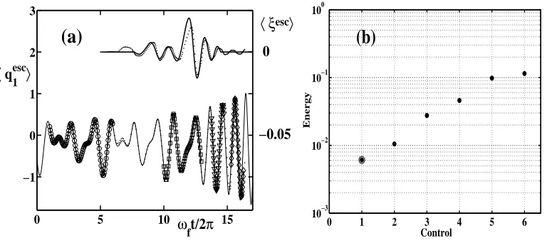
Once boundary conditions are specified one can solve the corresponding boundary value problem for the system (19) numerically.34 The results of the numerical solution of the boundary value problem obtained by the relaxational method are shown in Fig. 3(a) by the dotted lines and are in a good agreement with the solution found from the analysis of fluctuational trajectories. To demonstrate that the optimal force ˜u(t) found in the experiment really does minimise the energy of the control function steering the system (17) from the CA to the SC1 we set it to arbitrary initial conditions in the basin of attraction of the CA and let it evolve deterministically until it passed through the initial part of the unstable manifold of S5. At this moment the deterministic control function was switched on. For a given shape of the control function and/or initial conditions, its amplitude was set to the threshold for switching of the system from chaotic to regular motion on SC1.
It was found that the system is very sensitive to small variations in the control function: any deviation from the shape of ˜u(t), or from the initial conditions found in the experiment, leads to a substantial increase in the energy required to attain SC1. Some experimental results are shown in Fig. 3. It can be seen that the energy of the control function is approximately twice larger if the optimal force is approximated by the sin function modulated by a Gaussianu(t) =a1sin(a2t) exp(−(t−a3)2a4), and it is respectively∼4 and∼20 times
larger if the optimal force is approximated by rectangular pulses or distorted with an arbitrary low-frequency perturbation.
0 5 10 15 −1
0 1 2 3
ωft/2π
〈 q 1 esc〉
〈ξesc〉 0
(a)
−0.05
0 1 2 3 4 5 6
10−3 10−2 10−1 100
Control
Energy
[image:9.595.118.502.74.245.2](b)
Figure 3.(a)The most probable escape path (bottom solid curve) from S5 to the S1, found in the numerical simulations. Single periods of the unstable saddle cycles of period 5, 3 and 1 are shown by open circles, squares and triangles respectively; the stable limit cycle is shown by rombs. Parameters wereh= 0.13,ωf ≈0.95,ω0≈0.597,D≈0.01. Optimal force (top curve) corresponding to the optimal path after filtration. (b) Energies of various control functions used in the numerical experiments: 1 - optimal force found by statistical analysis of the fluctuational escape trajectories; 2 - approximation of the optimal force by u(t) =a1sin(a2t) exp(−(t−a3)2a4) whereaiare constants; 3 - approximation of the optimal force by the rectangular pulses; 4 - arbitrary perturbation of the optimal force with a low-frequency perturbation; 5 - control functions produced by the OPCL algorithm.
optimise the recovery time, rather than to minimise the energy of the control function, they are efficient in entraining the system dynamics to the goal dynamics. So it is interesting to compare their performance with that of the control function found in our experiment. The energy of the control functions (see Fig. 3(b)) obtained by these methods is more than an order of magnitude larger then the energy of the optimal control function ˜u(t) found by our new technique.
The results of this section demonstrate41 that a novel technique for the energy optimal steering of a chaotic system can be developed using the Hamiltonian formalism for the analysis of fluctuational trajectories in complex nonlinear systems.
5. NONLINEAR DYNAMICAL INFERENCE OF A CHAOTIC SYSTEM
As we have mentioned in the introduction, in the actual experimental situation the model is not usually known exactly from “first principles” and one is faced with the problem of inferencing a parametric model from the measured time-series data. For a complex stochastic nonlinear system this problem does not have a general solution.
Deterministic inference techniques3 consistently fail to yield accurate parameter estimates in the presence of noise. The problem becomes even more complicated when both measurement noise as well as intrinsic dynamical noise are present.42 A standard approach to this problem is often based on optimization of a certain cost function (a likelihood function) at the values of the model parameters that best reconstruct the measurements. It can be further generalized using a Bayesian formulation of the problem.42, 43 Existing techniques usually employ numerical Monte Carlo techniques for complex optimization44 or multidimensional integration43 tasks. Inference results from noisy observations are shown to be very sensitive to the specific choice of the likelihood function.45 Consequently, the correct choice of the likelihood function is one of the central questions in the inference of continuous-time noise-driven dynamical models considered here.
approach guarantees correct choice of the likelihood function that provides optimal compensation for the noise-induced errors. For the full N-dimensional version of the algorithm and its application to an ensemble of coupled oscillators see,46 an example of application of this algorithm to the real data of physiological experiment is discussed in.47
Consider for the sake of simplicity a one-dimensional dynamical system subject to additive noise of the form
˙
x=K(x|c) +ξ(t), (20)
ξ(t)= 0, ξ(t)ξ(0)=Dδ(t),
where K(x|c) is the deterministic drift force, ξ(t) is the white zero-mean Gaussian noise and D is the noise intensity. We assume that the unknown deterministic force can be represented in the form
K(x|c) =
M
k=1
ckfk(x), (21)
where fk(x) are known base functions, andc = {ck} is a set of unknown coefficients that have to be inferred from experimental data.
Suppose that we can measure directly in the experiment the dynamical variablex(t) by sampling it on a time lattice ti = tin+i h (i = 0,1, . . . , N) with the step h= (tfn−tin)/N. Using path-integral approach outlined
in Sec. 2 conditional probability density function (PDF)L(x|c) of an observationx(t) for a given choice of the model parametersc can we written as
L(x|c) =Pst(x(t0)|c)F[x], (22)
where Pst(x|c) is a stationary PDF of the system (20) given in (5). Thus all the information about our system is now encapsulated in the likelihood function that relates observations to the dynamical process (20).
Suppose also that we can use a priory available information and an expert opinion about our system sum-marized in a so-calledpriorPDFp(c).
Given a set of observation summarized in the likelihood function (22) one can improve ana priori estimate of the model parameters taking advantage of the Bayes theorem
p(c|x) = L(x|c)p(c)
L(x|c)p(c)dc. (23)
Herep(c|x) is a so-calledposteriorPDF that contains the improved by observations information about the model parameters. The integral in the denominator in (23) insures that the posterior PDF is normalized. Clearly, Eq.(23) can be applied iteratively each time a new record of measurements is used: prior distribution in the next iteration is just a posterior distribution from the previous iteration. For sufficiently large number N of observations in x the posterior distribution p(c|x) becomes sharply peaked about certain parameter values c
corresponding to the most probable model of the system for a given measurement set.
Let us choose the priorp(c) in a Gaussian form
p(c) =
detA0
(2π)M exp
−1
2(c−c0)
TA
0(c−c0)
, (24)
wherec0is a vector with arbitrary initial values of parameters andA0is a diagonal matrix with arbitrary values
of diagonal elements. In particular, small values of diagonal elements ofA0will reflect the fact that initial values
of the model parameters are not known. Now we can rewrite the likelihood in the form
L(x|c) = (2πDh)−N/2exp
−R
D −
γ− α
D
c−cT B
2Dc
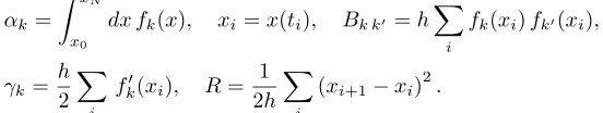
where
αk=
xN
x0
dx fk(x), xi =x(ti), Bk k =h
i
fk(xi)fk(xi),
γk= h2
i
fk(xi), R=21
h
i
(xi+1−xi)2.
Maximising the likelihood with respect to unknown model parameters we obtain the following algorithm of inference
Ap+1= B
D +Ap, cp+1=−A −1 p+1
γ− α
D −c
T pA
T
, (25)
where indexpcorresponds to prior parameters and indexp+ 1 corresponds to improved posterior parameters. Noise intensityD for each block of data can be inferred as
D= 2
N
i
R−αcp+cTpB2c
.
We now illustrate following47the application of the algorithm to inferencing a paradigmatic example of complex dynamical system – the Lorenz system. It has dynamical variables,x={x1, x2, x3}, the vector field
˙
x=σ(x2−x1),
˙
y=rx1+x2−x1x3,
z=x1x2−bx3.
(26)
and noise correlation matrix ξn(t)ξn(t)=dnδn,n. The parameters in (26) are σ= 10, r= 28, b = 83. We
10−2 10−1 10
(a)
0
101 102 −28 −14 0 14 28 t
〈 a
31〉 0.01 10 10−4 101 t 〈∆ a 2 31 〉 1 2 2 1
0 10 20 30 40 50
[image:11.595.177.453.93.145.2]0 40 80 120 r ρ
(b)
(r)Figure 4.(a) Examples of convergence of the coefficienta31 corresponding to parameterrof the Lorenz system (26) for the total length of the time recordT = 560 and the following sets of parameters: line 1{dn}={0.01,0.012,0.014}time steph= 0.002; line 2{dn}={100,120,140}andh= 0.00002. The insert shows dispersion∆a231=a231-a312 for the same sets of parameters. The vertical dashed line shows the time-scale of the step-wise decrease in the variance. (b) The comparison of the results of inference that take into account the prefactor term described in the text (black solid line) with the generalized least square fit (dotted line). The correct value of the coefficient is shown by vertical dashed line. To build distributionρ(r) of the inferred values of the coefficient r we have used an ensemble of 1000 numerical experiments using 90000 data points each. These results follow.47
sample a system trajectoryx(t) and produce a “data record” {y(tk)} to be fed directly into the algorithm. As
an inferential framework, we introduce the following model of stochastic dynamics forx(t):
˙
xn= 3
i=1
anixi(t) + 3
i<j=1
n, i, j = 1,2,3, where M ={{ani},{bnij},{Dn}} is the vector of 18 unknown coefficients and 3 values of the noise intensities. We note that for diagonal noise matrix as in the case of (27) the problem is reduced to 1D case of inference described in this section. We were able to infer the accurate values ofc,Dfor time stephvarying from 0.01 to 10−6 and noise intensitiesdn varying from 0 to 102. An example of convergence of the coefficients
is shown in Fig. 4 (see47 for further details).
We found a step-wise decrease in variances that occurs on a time scale of the period of oscillationsτosc≈0.6
(dashed line in the figure). The error of the inference is sensitive to the noise intensity, total timeT and the time steph. For example, for the parameters of the curve 1 in the Fig. 4 the relative error was 0.015%. The ratio
T /hhas to be increased at least 250 times to achieve error less then 1% when the noise intensity is increased 104 times (curve2 in the figure).
As show in47 it is important to keep the prefactor term in the probability density functional (5) to achieve correct results of inference. We demonstrate this following46 by comparing the statistical analysis of the results of inference of the coefficient r in the Lorenz equations preformed with and without prefactor term. As shown in the Fig. 4(b) the absence of this term results in a systematic underestimation of the model coefficient, while taking this term into account provides optimal compensation of the noise induced errors.
6. CONCLUSIONS
It is shown that novel effective techniques of prediction, control, and inference of complex dynamical systems can be addressed in a general framework of the path-integral approach to the analysis of the fluctuational trajectories.
ACKNOWLEDGMENTS
The work was supported by the Engineering and Physical Sciences Research Council (UK), NASA IS IDU project (USA), the Russian Foundation for Fundamental Science, and INTAS.
REFERENCES
1. R. Graham, A. Hamm, and T. Tel, “Nonequilibrium potentials for dynamical systems with fractal attractors or repellers,” Phys. Rev. Lett.66(24), pp. 3089–3092, 1991.
2. V. I. Mel’nikov, “The kramers problem: fifty years of development,” Physics Reports209(1/2), pp. 1–71, 1991.
3. H. Kantz and T. Schreiber,Nonlinear Time Series Analysis, Cambridge University Press, Cambridge, 1997. 4. S. Boccaletti, C. Grebogy, Y.-C. Lai, H. Mancini, and D. Maza, “The control of chaos: theory and
applica-tions,”Phys. Rep. 329, pp. 103–197, 2000.
5. M. I. Dykman and M. A. Krivoglaz, “Theory of the fluctuational transitions between the stable states of a nonlinear oscillator,” Sov. Phys. - JETP50, pp. 30–37, 1979.
6. M. I. Dykman, “Large fluctuations and fluctuational transitions in systems driven by colored gaussian noise–a high frequency noise,” Phys. Rev. A42, pp. 2020–2029, 1990.
7. R. Graham, “Path integral formulation of general diffusion processes,”Z. Phys. B26, pp. 281–290, 1977. 8. P. D. Beale, “Noise-induced escape from attractor in one-dimensional maps,”Phys. Rev. A40(7), pp. 3998–
4003, 1989.
9. Y. Kifer, “Large deviations in dynamical systems and stochastic processes,”Trans. Amer. Math. Soc.321(2), pp. 505–524, 1990.
10. R. L. Kautz, “Noise, chaos, and the josephson standard,”Rep. Prog. Phys.59, pp. 935–992, 1996.
11. P. Grassberger, “Noise-induced escape from attractors,” J. Phys. A: Math. Gen. 22(16), pp. 3283–3290, 1989.
12. R. Graham,Tracts in Modern Physics, vol. 66, ch. Quantum Statistics in Optics and Solid-State Physics. Springer-Verlag, New York, 1973.
14. A. J. McKane, “Noise-induced escape rate over a potential barrier: Results for a general noise,”Phys. Rev. A40(7), pp. 4050–4053, 1989.
15. D. Ludwig, “Persistence of dynamical systems under random perturbations,”SIAM Rev.17(4), pp. 605–640, 1975.
16. M. Freidlin and A. D. Wentzel,Random Perturbations in Dynamical Systems, Springer, New-York, 1984. 17. R. S. Maier and D. L. Stein, “Limiting exit location distributions in the stochastic exit problem,”SIAM J.
Appl. Math. 57(3), pp. 752–790, 1997.
18. V. N. Smelyanskiy, M. I. Dykman, and R. S. Maier, “Topological features of large fluctuations to the interior of a limit cycle,”Phys. Rev. E55(3), pp. 2369–2391, 1997.
19. M. I. Dykman, P. V. E. McClintock, V. N. Smelyanskiy, N. D. Stein, and N. G. Stocks, “Optimal paths and the prehistory problem for large fluctuations in noise driven systems,”Phys. Rev. Let.68(18), pp. 2718–2721, 1992.
20. D. G. Luchinsky, “On the nature of large fluctuations in equilibrium systems: observation of an optimal force,”J. Phys. A30(16), pp. L577–L583, 1997.
21. M. I. Dykman, D. G. Luchinsky, P. V. E. McClintock, and V. N. Smelyanskiy, “Corrals and critical behavior of the distribution of fluctuational paths,”Phys. Rev. Lett.77(27), pp. 5229–5232, 1996.
22. D. G. Luchinsky, R. S. Maier, R. Mannella, P. V. E. McClintock, and D. L. Stein, “Experiments on critical phenomena in a noisy exit problem,”Phys. Rev. Lett.79(17), pp. 3117–3120, 1997.
23. D. G. Luchinsky and P. V. E. McClintock, “Irreversibility of classical fluctuations studied in analogue electrical circuits,”Nature 389(6650), pp. 463–466, 1997.
24. D. G. Luchinsky, P. V. E. McClintock, and M. I. Dykman, “Analogue studies of nonlinear systems,”Reports on Progress in Physics61(8), pp. 889–997, 1998.
25. J. Hales, A. Zhukov, R. Roy, and M. I. Dykman, “Dynamics of activated escape and its observation in a semiconductor laser,”Phys. Rev. Lett.85(1), pp. 78–81, 2000.
26. R. L. Kautz, “Activation energy for thermally induced escape from a basin of attraction,” Phys. Lett. A
125(6,7), pp. 315–319, 1987.
27. J. Guckenheimer and P. Holmes,Nonlinearoscillations, Dynamical Systems, and bifurcations of vector fields, Springer-Verlag, New-York, 1983.
28. E. Ott,Chaos in Dynamical Systems, Cambridge University Press, Cambridge, 2002.
29. P. Holmes, “A nonlinear oscillator with a strange attractor,”Phil. Trans. R. Soc.292, pp. 419–448, 1979. 30. S. V. McDonald, C. Grebogi, E. Ott, and J. A. Yorke, “Fractal basin boundaries,”Physica D17, pp. 125–
153, 1985.
31. C. Grebogi, S. W. McDonald, and E. Ott, “Final-state sensitivity - an obstruction to predictability,”Phys. Lett. A 99, pp. 415–418, 1983.
32. C. Grebogi, E. Ott, and J. A. Yorke, “Basin boundary metamorphoses - changes in accessible boundary orbits,”Physica D24, pp. 243–262, 1987.
33. A. Silchencko, S. Beri, D. G. Luchinsky, and P. V. E. McCLintock, “Fluctuational transitions through a fractal basin boundary,”Phys. Rev. Lett.91, p. 174104, 2003.
34. D. G. Luchinsky, S. Beri, R. Mannella, P. V. E. McClintock, and I. A. Khovanov, “Optimal fluctuations and the control of chaos,”Int. J. Bif. Chaos12(3), pp. 583–604, 2002.
35. V. N. Smelyanskiy and M. I. Dykman, “Optimal control of large fluctuations,”Phys. Rev. E55(3), pp. 2516– 2521, 1997.
36. L. D. Landau and E. M. Lifshitz,Statistical Physics, Pergamon, New York, 3rd ed., 1980. Part 1.
37. L. Onsager and S. Machlup, “Fluctuations and irreversible processes,” Phys. Rev.91(6), pp. 1505–1512, 1953.
38. R. P. Feynman and A. R. Hibbs,Quantum Mechanics and Path Integrals, McGraw-Hill, New-York, 1965. 39. E. A. Jackson, “The oplc control methods for entrainment, model-resonance, and migration actions on
multiple-attractor systems,”Chaos7(4), pp. 550–559, 1997.
41. I. A. Khovanov, D. G. Luchinsky, P. V. E. McClintock, and R. Mannella, “Fluctuations and the energy-optimal control of chaos,”Phys. Rev. Lett.85(10), pp. 2100–2103, 2000.
42. R. Meyer and N. Christensen, “Fast bayesian reconstruction of chaotic dynamical systems via extended kalman filtering,”Phys. Rev. E65, p. 016206, 2001.
43. R. Meyer and N. Christensen, “Bayesian reconstruction of chaotic dynamical systems,” Phys. Rev. E 62, pp. 3535–3542, 2000.
44. J.-M. Fullana and M. Rossi, “Identification methods for nonlinear stochastic systems,” Phys. Rev. E 65, p. 031107, 2002.
45. P. E. McSharry and L. A. Smith, “Better nonlinear models from noisy data: attractors with maximum likelihood,”Phys. Rev. Lett.83, pp. 4285–4288, 1999.
46. V. N. Smelyanskiy, D. G. Luchinsky and R. Morris, “Inference of stochastic nonlinear oscillators with applications to physiological problems,” see this issue of SPIE proceedings.