Munich Personal RePEc Archive
Procurement auctions with avoidable
fixed costs: an experimental approach
Larson, Nathan and Elmaghraby, Wedad
University of Virginia
2008
Online at
https://mpra.ub.uni-muenchen.de/32163/
Procurement Auctions with Avoidable Fixed Costs: An
Experimental Approach
Wedad Elmaghraby∗ and Nathan Larson†‡
January 11, 2011
Abstract
Bidders in procurement auctions often face avoidable fixed costs. This can make bidding decisions complex and risky, and market outcomes volatile. If bidders deviate from risk neutral best responses, either due to faulty optimization or risk attitudes, then equilibrium predictions can perform poorly. In this paper, we confront laboratory bidders with three auction formats that make bidding difficult and risky in different ways. We find that measures of ‘difficulty’ pro-vide a consistent explanation of deviations from best response bidding across the three formats. In contrast, risk and loss preferences cannot explain behavior across all three formats.
Keywords: Auctions, Experimental, Procurement, Synergies, Asymmetric Bidders, Learning, Optimization errors
1
Introduction
Procurement auctions are often used in settings where suppliers have avoidable fixed costs (El-maghraby (2007)). Prior experimental studies have showed that bidding and auction outcomes in such settings can be quite volatile, and that convergence to equilibrium predictions may be poor. In this paper, we use experiments to study the reasons that suppliers deviate from risk neutral best response bidding when avoidable fixed costs are present. In particular, we ask whether these deviations are better explained by preferences (e.g., suppliers who are not risk neutral) or by opti-mization errors. To address this question, we study bidding in three auction formats across which the level of payoff risk and the difficulty of optimization vary. Our main finding is that measures of optimization difficulty help to explain behavior across auction formats. In contrast, our preference-based explanations do not generalize well across auction formats – while they may be helpful in
∗The Robert H. Smith School of Business, University of Maryland, College Park, MD 20742. Email:
†Department of Economics, University of Virginia, Charlottesville, VA. Email: [email protected]
‡This paper has benefited greatly from the comments provided by seminar participants at UCLA, University of
understanding bidding under one set of rules, they do not offer reliable guidance about what to expect when the rules change.
Avoidable fixed costs are fixed production costs that a supplier does not incur unless it sells a strictly positive quantity. This makes costs non-convex: the marginal cost of the first unit sold may be higher than that of additional units. One result of this is that small, marginal changes can have large, non-marginal consequences. For example, in an efficient allocation, a small cost rise for one supplier may cause it to be dropped from the allocation completely (rather than having its quantity decline gradually). Furthermore, prior research shows (e.g. Van Boening and Wilcox (1996) and Van Boening and Wilcox (2005)) that even when supplier costs are stable, market prices and allocations can remain volatile rather than settling down toward equilibrium. To some extent, the first point may be directly to blame for the second. Any auction format that aspires to be efficient must be willing to make large changes to the winning allocation in response to small changes in bids. However, this may confront bidders with risks they prefer to avoid or with strategic challenges that confound learning.
We select three auction formats for which we expect the difficulty of optimization and the level of payoff risk to differ. In all three formats, suppliers have (private) average costs that are either increasing, constant, or decreasing, and a supplier can produce either zero, one, or two units. We intepret the decreasing average cost case to represent a supplier with an avoidable fixed cost. For such a supplier, selling at certain prices will be profitable only if she sells her full capacity. In the first auction format (1U)1, each supplier submits a single bid specifying the lowest per-unit price it is willing to accept. Bids are ranked in increasing order, and the auction clears at the lowest uniform price that procures the total desired quantity. The second auction format (2U) retains a uniform price, but allows suppliers to fully express their costs with quantity-dependent bids. In the third format (2D), both bids and prices are quantity dependent. Each format presents some idiosyncratic features. For example, in 1U equilibrium bidding is inherently unstable (in the sense that some bidders must use mixed strategies) and requires some suppliers to bid well below cost and hope for a favorable price and quantity. In 2U, optimal bids are simple but not particularly intuitive – they may elude a subject who is not prepared to experiment with different bids. In 2D, while the winner determination process is complex, equilibrium (for our parameters) tends to segment competition into sub-markets at different quantities. A subject who treats these sub-markets as independent errs only slightly, and this substantially simplifies the strategic problem she faces.
First we test how well equilibrium outcomes (such as efficiency and total procurement cost) predict actual outcomes across these environments. The equilibrium predictions are fairly successful for 2D, but less so for 1U and 2U, suggesting that there are persistent deviations from risk neutral best response bidding. To assess those deviations, we compute empirical best response profits for each subject; these are the profits that a subject would have earned in each auction by best responding to the empirical distribution of bids that he had faced in the past. Since a subject does not face equilibrium bids from opponents, these empirical best response profits provide a
1
more reasonable benchmark than equilibrium payoffs do for the amount that a risk neutral best responder could have earned. In treatment 2D, the actual profits earned by subjects were close to these benchmark profits. However, in the other two environments, actual payoffs are below these benchmarks on average, and do not track them closely from auction to auction.
This leads us to try to develop a unified model of bidding that can explain why bids are close to risk neutral best responses in 2D but deviate from them in the other two treatments. We construct and estimate a learning model in the spirit of Erev and Roth (1998) and Camerer and Ho (1999). In the model, a subject’s propensity to pick a particular bid evolves in response to her market experience. Propensities map into probabilities of choosing different bids according to a standard logit formulation. The propensity includes a term for the expected profit that the bid would have earned against past opponents; a subject choosing on this basis alone would play a risk neutral best response. We also allow this propensity to depend on factors that are intended to capture alternative preferences or the difficulty of optimization. We test the robustness, or generality, of these preference and optimization-based explanations by fitting models to two of the three auction formats and then predicting bids in the third format.
We focus on three potential sources of optimization difficulty: volatile feedback, difficulty of the payoff landscape, and non-separability of the bidding problem. Volatile feedback, or ‘noisy optimization,’ captures the idea that a supplier may have trouble discerning the expected payoff of a bid when the bid’s realized payoff varies a lot. By ‘landscape difficulty’ we mean the idea that a payoff function shaped like Mt. Everest may be easier to maximize than one shaped like San Fran-cisco (many local maxima) or like Kansas (long flat stretches). As one might imagine, formalizing this notion poses its own challenges, and we defer discussing our results for this explanation until later. By ‘separable,’ we mean a bidding problem that can be tackled effectively by decomposition into smaller pieces. We also study a factor that could aid optimization - namely the fact that some strategies are weakly dominated and others are not. For preference-based explanations of bidding, we concentrate on simple formulations of risk and loss aversion.
In some cases we can compare the preference and optimization-based explanations head to head. Both the noisy optimization story and risk averse preferences imply that a bid’s payoff variability (defined as the variance of its payoff against a subject’s past opponents) should affect how often it is chosen. However because the predicted effects are different, we can compare these explanations in the data. We find that risk aversion cannot provide a consistent explanation of bidding across all three auction formats. In contrast, a single model of noisy optimization explains patterns within and across auction formats rather well.
Next we set weak dominance and loss aversion head to head. All bids below cost, which we call loss exposed, have the potential to lose money. Some of these loss exposed bids are also weakly dominated, while others can be profitable, or even optimal, on average.2 We test whether (i) subjects avoid all loss exposed bids or (ii) subjects specifically avoid weakly dominated bids. Both (i) and (ii) help to explain bidding, but the predictions of (ii) are more robust across auction
2
formats. We infer that loss attitudes, if present, are unstable. From (ii) we learn that among bids with low expected payoffs, subjects are better at avoiding the “sure losers” than bids with some chance of an upside.
For both the risk and loss-based models, poor robustness is related to major behavior differences between formats 1U and 2U. In the latter, subjects avoid modestly risky or loss exposed bids, even when the potential payoff gains are large. In the former, subjects favor quite risky bids, even though the payoff gains they offer are small or even negative. Thus, while risk and loss attitudes may be helpful in understanding bidding under one set of rules, they do not offer reliable guidance about what to expect when the rules change.
With regard to separability, in our setup most allocations will involve one two unit supplier and one one unit supplier. It could be tempting for subjects to try to simplify the bidding problem by treating these as separate and independent market niches. To test this, we decompose a bid’s expected payoff into portions earned by winning one or two units respectively. Then we enter these two terms separately in the propensity to bid equation. We find that subjects consistently focus on either one unit profits or on two unit profits, ignoring the possibility of gains or losses from winning the other quantity. We argue that this “two separate submarkets” shortcut is closer to the truth in format 2D than in the other auction formats, and this contributes to better profit maximization by subjects in 2D.
Concentrating on expected profits from one submarket is an example of a heuristic that subjects use to simplify bidding. However, even this may be difficult: it requires subjects to understand winner determination well enough to estimate counterfactual market outcomes. Motivated by models of reinforcement learning, we also test for simpler a simpler heuristic: does a subject simply reinforce bids that have won her a particular quantity in the past? We incorporate ‘quantity reinforcement’ terms into the propensity to bid equation (allowing for spillover reinforcement to nearby bids). These terms let us test for three types of goal-oriented behavior: local inertia (a tendency to stay near any bids used previously), win targeting (favoring any bids that have won positive quantities), and competitive quantity targeting (favoring bids that win the quantity the subject can produce at least average cost). We find that inertia is quite strong in all three auction formats. This serves subjects well in format 2D – their instincts about where to start bidding (cost plus a markup for each quantity) are basically correct and require only local fine-tuning. However, in the other two formats, their initial intuition about how to bid is less accurate, and inertia leads them to overlook opportunities to improve. We also find evidence of quantity targeting, suggesting that subjects use it as a low tech proxy for identifying profitable bids.
In Section 2 we position our contribution relative to related work on markets with non-convex preferences and learning to optimize in complex environments. Section 3 describes our model, auction formats, and experimental procedure. Section 4 presents session-level comparisons of ex-perimental outcomes with theoretical predictions. Section 5 introduces our models of the individual bidding decision, and Section 6 presents results for these models. In Section 7, we test the quantity reinforcement heuristics. We conclude with some suggested directions for future work.3
3
2
Context and Related Work
Avoidable fixed costs are relatively common in procurement; for example, when goods or services are produced to order, there is often a start up cost related to setting up a production line or training employees to handle customized aspects of the order. Wholesale electricity procurement provides a nice illustration of the complications this can cause, and also of competing views about how they should be handled. With certain types of power plants, a start-up cost is incurred whenever an idle plant is called into service. In the original design of the California Power Exchange (one of the earliest deregulated electricity markets in the U.S.), bids allowed suppliers to express variable cost but not to separately express start-up costs. Market clearing involved a simple ranking of bids, with all winning bidders receiving the same uniform price. Because a marginal supplier could be rationed, a supplier faced the risk of not winning a large enough quantity to recoup its start-up cost. In this market, the task of trying to bid competitively enough to win while avoiding this exposure risk was shouldered by the bidders.
In contrast to California, the Pennsylvania-New Jersey-Maryland (PJM) market (the largest competitive wholesale electricity market in the world) allows suppliers to submit multi-part bids, so that it is possible to express both start-up and variable costs. These bids are fed into a com-plex optimization procedure which determines the winning allocation and sets what amount to bidder-specific prices.4 This format makes a bidder’s decision problem simpler in some respects
(it is easy ensure that one’s costs are covered) but harder in others: bidding optimally requires an understanding of how one’s bid will affect market outcomes (prices and allocations), and the optimization procedure can make this rather opaque. Studying how bidders handle a more opaque allocation procedure without exposure risk, relative to a more transparent allocation where expo-sure risk is severe, is one object of our comparison between formats 1U and 2U and 2D.
Avoidable fixed costs may be thought of as a type of cost synergy, since a supplier’s per unit cost may be lower at larger quantities. There is also a closely related experimental literature on standard (i.e. forward) auctions in which bidders have demand synergies. Katok and Roth (2004) study the decisions of a single large bidder with a demand synergy for two units, who competes against several small (one unit) bidders who follow simple dominant strategies. In an ascending price format where the large bidder faces exposure risk, they find that this bidder bids too cautiously (relative to his risk neutral best response), depressing the seller’s revenues (relative to equilibrium). They also study a descending price auction that gives the large bidder more control over its quantity, thus eliminating exposure risk. They find that in this format, the large bidder suffers fewer losses and allocative efficiency is higher. Our experiment also features small and large bidders, with large bidders subject to exposure risk, but there are a number of major differences. Most importantly, we allow for competition among more than one large bidder; this makes it substantially more difficult for bidders to anticipate both how their opponents will bid, and how their own bidding will affect the winning allocation. We also test whether subjects’ responses to exposure risk are
an online appendix at http://people.virginia.edu/ nl2a/Papers/Submitted/lumpy-code.html .
4
consistent across different settings (1U and 2U). Another difference is that our auction formats are static rather than dynamic. Like Katok and Roth, we find more efficient allocations when bidders can make quantity dependent bids (2D and 2U versus 1U), but in our case, fear of exposure does not explain departures from best response bidding very consistently.
Our work is close in spirit to a sequence of three papers by Van Boening and Wilcox (1996 and 2005, henceforth VBW) and Durham et al. (1996). These papers share an experimental design in which multiple buyers (3 or 4) and suppliers (3 or 4) trade in a double auction format. All suppliers have zero variable cost and positive avoidable fixed costs; “larger” suppliers have larger fixed costs and larger capacities. The mix of supplier types is the same in each auction. In VBW (1996), suppliers were restricted to making a single, per unit bid and were paid a uniform price if selected for production. Prior studies have shown this mechanism to be highly efficient when supplier costs are convex. However, with avoidable fixed costs, VBW find a “roller coaster” between efficient and inefficient outcomes that does not settle down as subjects become more experienced. The volatility of outcomes occurs even in parameter configurations for which a competitive equilibrium (at a uniform price) exists. Interesting, they observe a tendency for bids to converge to a single uniform price, even in settings where the only possible competitive equilibrium would require nonlinear prices.
Durham et al. (1996) study whether a richer strategy space for bidders can encourage con-vergence to efficient outcomes and equilibrium prices in the double auction. They allow suppliers to bid a two-part tariff (a fixed amount if selected to produce, plus a per unit price) and to set an upper bound on the number of units supplied. Despite the expanded bid space, the authors find that the volatility of market outcomes persists and that those outcomes are rarely to never consistent with equilibrium.
VBW (2005) expanded the bidding space further to allow suppliers to offer (a limited number of) price-quantity contracts. (This is their “BUDA” auction format.) One aim was to determine whether suppliers were able to converge to an efficient equilibrium supported by quantity-dependent prices. They found a modest improvement in efficiency (relative to a standard double auction), but persistence of linear (not quantity-dependent) prices. Thus, the evidence about whether the BUDA rules nudge the market toward an equilibrium outcome is mixed. In a variation (RBUDA), one unit contracts were forbidden to see whether the market’s tendency toward a (non-equilibrium) uniform price could be broken. (One rationale would be that, by facilitating arbitrage between contracts of different quantities, one unit contracts tend to linearize prices.) VBW found that this restriction does promote convergence to quantity-dependent pricing, but does not improve efficiency (relative to BUDA). Since the equilibrium outcome is efficient, it is unclear whether the RBUDA rules pushed the market closer to equilibrium outcomes.
Like these three papers, we study markets with avoidable fixed costs on the supply side, but we study static auctions with a single buyer, not double auctions. We also differ in that our suppliers have a range of convex and non-convex cost structures, and compared to the two VBW papers, bidders are observed over more auction rounds.5 Like these earlier papers, we also find volatility
5
in our market outcomes. However, we diverge from this earlier work by attempting to explain the divergence between actual and equilibrium market outcomes using models of the individual’s bidding decision.
While models of bounded rationality and imperfect optimization are common in the economics literature, less attention has been paid to the features of a strategic decision problem that make it hard. Our metrics of difficulty in this paper are partially motivated by a broad literature on this question outside of economics. In the context of a decision task under adverse selection, Bereby-Meyer and Grosskopf (2008) cite extensive evidence that subjects do not learn to avoid bad decisions when payoff variability is high. In a manipulation where payoff variability is reduced, they show that learning improves substantially.
If one treats a payoff function as a ‘landscape’ traversed by subjects in search of the highest peak, many candidate notions of what constitutes a hard landscape have been proposed, none entirely satisfactory. Jones and Forrest (1995) discuss the challenges of finding a metric that can classify both ‘rugged’ problems (e.g. San Francisco) and ‘needle in a haystack’ problems (e.g. a landscape with one ice cube atop an ice rink) as hard. We propose a simple metric based on counting local maxima that can capture both of these notions of difficulty in our setting.
Finally, there is a multi-disciplinary literature on separability (often referred to as decomposi-tion or modularity) of objective funcdecomposi-tions spanning evoludecomposi-tionary biology, genetic algorithms, and management. This work can be hard to translate into economics, but Page (1996) suggests a mea-sure of difficulty based on decomposing an objective function into as many independent subproblems as possible and reporting the size of the largest subproblem. (For a non-modular objective, this largest subproblem might simply be the original problem itself.) We will argue that under an in-formal interpretation of this criterion, the bidding problem is approximately separable in 2D but not in the other two treatments.
As we suggested in the introduction, subjects may attempt to decompose the bidding problem into simpler pieces even when this is not a suitable tactic. In a different context, Ashby et al. (1999) confront subjects with a two-dimensional categorization task. They find that subjects tend to rely on simple, one-dimensional classification rules, regardless of whether this is optimal. This is similar to our finding that even though optimal bidding can require tradeoffs across two outcome dimensions (payoffs from winning one unit versus winning two units), our subjects appear to simplify the problem by simply ignoring one of these dimensions.
3
The Experimental Environment
3.1 Demand and Supplier Costs
There is a single buyer who demands D= 3 discrete units of a good. If necessary, it can produce the good in-house at constant marginal cost R = 100; D and R are commonly known constants. The buyer faces three suppliers whose roles are played by subjects in the experiment. Each supplier can produce either 0, 1, or 2 units of the good. A supplier’s average cost of supplying q units is given bycq, where
c0 = 0 c1 = 100−θ c2 =
100 +θ
2 .
A supplier’s cost parameter θ, which indexes the convexity of its costs, is private to the supplier. A large value of θ indicates increasing average (and marginal) cost, while a supplier with θ small can supply two units at a lower per unit cost than one unit. If θ= 3313, the supplier has constant marginal cost. In the background, one may think of the case c2 < c1 as a consequence of a
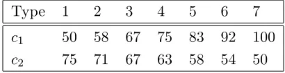
large avoidable fixed cost, but this interpretation is not essential to the analysis. In solving for equilibrium, we treat θ as drawn uniformly from [0,50], but in the experiments we discretize this range to seven evenly spaced types, denoted byc1 ∈ {50,58,67,75,83,92,100}.
This setting is designed to capture, as simply as possible, certain features that make the supply allocation problem interesting. First, there is a mix of efficient production scales – small (large) suppliers minimize per unit cost when producing one (two) units – and none of the cost types is strictly dominated by any other type. Second, an allocation will generally require participation from at least two suppliers at different quantity levels – in this case, two units from one supplier and one from another. Furthermore, an efficient allocation typically requires one large supplier and one small one to win.6 Partly as a consequence of this, efficiency cannot be determined by at
the margin – a cost-minimizing allocation must consider both marginal and inframarginal costs. Using the one-dimensional index θpermits us to incorporate these features in a parsimonious and relatively tractable way.
3.2 Experimental Procedure
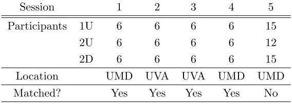
The experiments were conducted with undergraduate students in the Netcentricity Behavior Lab at the University of Maryland (UMD) and the vEconlab at the University of Virginia (UVA). There were three treatments, 1U, 2U, and 2D, corresponding to the three auction formats described in the next section. For each treatment, there were five independent sessions (Sessions 1 to 5) with six participants in each session.7 Details are summarized in Table 1. Each subject earned a show-up
fee of $10, which also served as an initial balance to which any profits or losses during the session were added.8 Earnings during the session were measured in an experimental currency (‘francs’) and
6
Production of one unit by all three suppliers is also a possibility, but given the avoidable fixed costs, it is rarely efficient.
7
Session 5 had more participants – see Table 1 for details.
8
Session 1 2 3 4 5
Participants 1U 6 6 6 6 15
2U 6 6 6 6 12
2D 6 6 6 6 15
Location UMD UVA UVA UMD UMD
[image:10.612.164.448.74.176.2]Matched? Yes Yes Yes Yes No
Table 1: Summary of Experimental Sessions
were later converted to dollars at the rate of 50 francs to $1 USD. Upon arrival, subjects were given written instructions which were read aloud by the experimenter. Then subjects participated in three practice (non-paying) rounds of auctions to familiarize them with the experimental software.9 At this point, there was a pause to answer any questions; then the live (paying) rounds began.
The experimental phase of each session consisted of 30 rounds. In each round subjects were randomly matched in groups of three to compete in an auction. At the start of Rounds 1, 7, 13, 19, and 25, each subject drew a private cost type independently and uniformly from the seven types shown in Table 2. 10 We refer to cost typesc1∈ {50,58,92,100}asspecialized types and cost types
c1 ∈ {67,75,83}asflexible types. Informally, we will refer to a supplier as small or large depending
on whether c1 ≤ c2 or c1 > c2, but in certain parts of the data analysis we restrict small to be
{50,58} and large to be {92,100} (with the remainder of types as flexible). A subject kept the same cost type for a block of six rounds, called asub-session, before drawing a new type. Both the random matching and the random sequence of cost draws were matched, session by session, across treatments. (That is, for Sessioni, a full sequence of cost types was drawn and matched into groups of three over thirty rounds. This sequence was then used for Sessioniof all three treatments.)11
At the end of each round, subjects were shown: (i) their costs, (ii) their bid(s), (iii) how many units they won in that round, (iv) the winning price(s), (v) their profit in that round, and (vi) their cumulative profit including the $10 show-up fee. Each session ran for about 90 minutes, start to finish, and subjects were paid immediately upon completion of the session.
smallest final payoff for any subject was approximately $7.
9
The experiment was programmed and conducted with the software z-Tree (Fischbacher 2007).
10
The types are only approximately spaced betweenθ= 0 andθ= 50 because costs are rounded to integers. Note also that there are no “round” numbers in the cost table (multiples of 5 or 10) by design. Our pilots indicated that round costs tended to produce bids that were also anchored to multiples of 5 or 10, an artifact that we wanted to avoid.
11
Type 1 2 3 4 5 6 7
c1 50 58 67 75 83 92 100
[image:11.612.203.408.73.126.2]c2 75 71 67 63 58 54 50
Table 2: Supplier Cost Types
3.3 Auction Formats
In this section we introduce our three auction formats, the nature of the bidding challenge in each auction and characterize (approximate) equilibrium behavior in these markets. In our characteriza-tion of the equilibrium, we take it as given that subjects are racharacteriza-tional, risk-neutral profit maximizers. Embodied in rationality are the ideas that subjects perfectly understand the strategic environment, develop correct beliefs about the bidding of opponents, and do not consistently miss opportuni-ties to improve their payoffs. This allows us to make a “best-case” evaluation of how successfully each auction provides incentives that align individual profit-seeking with efficient allocation and competitive bidding.
3.4 1U : One-part bids, uniform pricing (1U)
Under 1U, each bidder simultaneously submits a one-dimensional bid b. This bid is a pledge to make its entire capacity, or any part of it, available at any price per unit greater than or equal to
b. The buyer procures the entire capacity of the lowest bidder (in this case 2 units from the lowest bidder) and the remaining one unit from the next lowest bidder. All bidders are paid a uniform price per unit equal to the bid of the marginal winning bidder (that is, the second lowest bidder). For example, if three suppliers submitted bids of 70, 80, and 85, the allocation would be two units for the first supplier and one unit for the second, and both winners would be paid 80 per unit.
Variations on this simple uniform price auction format are common in practice, and when supplier costs are convex, its (theoretical) efficiency can be high, since the uniform price tends toward equating the costs of the marginal unit procured from each bidder. However, with avoidable fixed costs, a supplier’s willingness to supply at a particular price may depend on the quantity it will be asked to produce, but there is no way to express this through the bidding. Hence, bidders in 1U confront both quantity risk and price risk. Quantity risk reflects the fact that any given bid could turn into an obligation to produce either zero, one, or two units, regardless of the intent of the bidder. A large bidder who bids intending to win two units may only win one and fail to cover its costs ( illustrating the exposure problem), or a small bidder who intends to be marginal may wind up inframarginal, obligating it to produce an unprofitably large quantity. Bidding lower monotonically improves one’s chances of winning two units, and has a non-monotonic effect (first rising, then falling) on the chance of winning one, so there are several different tradeoffs for a bidder to consider as it tries to maximize its expected profit.
arising from the fact that its price is set the next lowest rival bid. What is less obvious is that in order to be competitive for two units (and avoid winning one), a large bidder may need to bid below its two-unit average cost. Thus, it can end up losing money with its optimal bid, even if it wins its desired quantity, when the price-setting bid is low enough.
This rich set of tradeoffs has two important implications for bidder behavior. First, these incentives interact in such a way to preclude the existence ofany pure strategy equilibrium – any equilibrium involves mixing by some cost types (discussed below).12 Second, it allows us to test the implications of risk aversion in a much more nuanced way than is typically possible.
An analytical characterization of the mixed strategy equilibrium is intractible, but we can compute equilibrium strategies numerically for both the continuous and discrete type cases. Figure 1 shows these strategies (presented as cumulative distribution functions over bids) for the discrete case.13 The smallest suppliers (c1 ∈ {50,58}) concentrate at b = 69. The largest supplier types
(c1 ∈ {92,100}) mix over a compact range of bids. However, each flexible type mixes over two
separate intervals, one with low bids and one with high bids.
If one of these flexible types were to always bid in the higher of these two intervals, then market prices would tend to be higher, and any individual supplier of this type would be tempted to try to win two units at a high price by deviating to a low bid. Conversely, if one of these flexible types were to always bid in the lower of the two intervals in its support, then prices would tend to be lower, reducing inframarginal profits. In this case, an individual of this type could do better by abandoning hope of winning two units and deviating to a high bid that might set the price. Thus equilibrium requires these types to mix between bids that are more competitive for the inframarginal and marginal units, respectively.
3.5 2U : Two-part bids, uniform pricing (2U)
Under 2U, the bidding space is expanded to reflect the supplier’s cost structure, but all units continue to be paid the same uniform price. Each bidder submits a two-part bid (b1, b2) indicating
the minimum priceper unit it is willing to be paid if it supplies one unit (b1) or two units (b2). The
market-clearing price is defined to be the lowest price at which it is possible to procure exactly three units by fulfilling some subset of the submitted bids, taking at most one bid from each supplier. If there is only one subset of bids that achieves this, then it becomes the winning allocation. If more than one subset of bids could provide exactly three units at the market-clearing price, then a tiebreaker is needed. We break ties in favor of the allocation whose cost would be lowest if
12
This is true both with the continuous type space, and with the discretization to seven types.
13
the suppliers were paid as bid.14, 15By introducing dependent bidding without
quantity-dependent pricing, 2U is in some sense creating two markets but leaving one of them unpriced. This makes bidding less risky, since a supplier can guarantee that its costs will be covered, but it also makes the auction price a less effective signal to suppliers about how to bid successfully.
Below we present equilibrium bidding strategies under 2U for the version of our model with continuous costs. Simulations suggest that this equilibrium is both unique and a qualitatively accurate approximation of equilibrium with discrete cost types.16 The symmetric equilibrium bids, as a function of one-unit cost c1 are
b1(c1) =
(
3c1+ 100 ln (1−c1/100) + 100 ln 3−100 if c1 ≤ 2003 ≈66.7
100 ifc1 > 2003
b2(c1) = 0
The proof that these strategies constitute an equilibrium is in Appendix A; below we provide intuition behind the equilibrium.
Note that one unit bids are above 90 for all types and all types between c1 = 67 andc1 = 100
pool at 100. Meanwhile, two unit bids are pooled at zero. To better understand this ‘highball-lowball’ bidding strategy result, observe that if these strategies are followed, the price will always be set by a (very high) one unit bid, and the lowest two unit bidder will supply two units at this price. Given these strategies, the price will be high enough that it is attractive to all cost types – even c1 = 50 – to try to submit the lowest b2 and sell two units. Since submitting a lowball b2
bid is essentially costless – in equilibrium it never turns out to set the price – this undercutting incentive sendsb2 down to the lowest permissible bid, which is zero.
14
To illustrate, suppose that the three suppliers submit bids of (70,77), (75,71), and (100,55). At prices below 70, it is only possible to procure a total of two units, both from the third supplier. At a price of 70, it is possible to procure one unit from the first supplier and two units from the third, so this is the winning allocation, and the market-clearing price is 70. Now change the second supplier’s bid to (75,60), holding the other bids fixed. At prices in [60,70) it is possible to procure either two units (from either the second or third supplier) or four units (two from both), but not exactly three. At a price of 70, there are two ways to procure three units: one unit from the first supplier and two units from either the second or the third. The market-clearing price is again 70, and the tie is broken in favor of the allocation including the third supplier (70 + 2 (55)<70 + 2 (60)). This outcome involves passing up a bid below the market-clearing price (the second supplier’s two unit bid) in order to procure exactly the quantity demanded by the buyer. Notice that the second supplier could enter the winning allocation here by undercutting the third supplier’s two unit bid, and that this would have no effect on the market-clearing price.
15
This allocation rule – consistent with the instructions provided to subjects – precludes the possibility that the buyer accepts a two unit bid but asks its bidder to deliver only one unit. We thank a referee for pointing out that if the buyer did have this option, then it might sometimes be advantageous to procure three units by accepting two different two unit bids, paying for all four units, but only taking delivery of three. While the equilibrium strategies would certainly change in this case, the chance of being paid for an unproduced and undelivered second unit would still tend to induce bidding below cost.
16
This equilibrium does not make format 2U look very attractive: equilibrium efficiency should be low because of the pooling and procurement cost should be quite high. However, our goal is not to identify optimal auctions but to examine how successfully suppliers can master a difficult bidding problem. Format 2U delivers such a problem: to do well, a subject must break free from the intuition that a good bid should be in the neighborhood of a markup above her costs.
3.6 2D: Two-part bids, discriminatory pricing (2D)
Under 2D, a bidder submits a two-part bid (b1, b2), as under 2U. However, under 2D, each supplier
is paid the amount of its own accepted bid per unit supplied. A supplier’s bids are still mutually exclusive: a supplier will either haveb1 accepted, supply one unit, and be paidb1, or it will haveb2
accepted, supply two units, and be paid a total of 2b2, or it will have no bid accepted and produce
zero. The winning allocation is determined by accepting the combination of bids that procures exactly three units at the least total cost to the buyer, subject to the constraint that at most one bid is accepted from each supplier.17
An approximation of symmetric equilibrium bidding strategies, as a function of one-unit cost
c1 are,
b1(c1) =
100
3 +
2 3c1
b2(c1) = 11
12100− 1
3c1 = 25 + 2 3c2
The bidding strategies above are an exact equilibrium for the model with continuous cost types, under the assumption that only two bidder allocations are permitted. The strategies are only approximately optimal if three bidder allocations are permitted, but because three bidder allocations only occur in around one in thirty auctions, the approximation is quite close.
These bidding strategies leverage the fact that under our cost structure, a supplier’s one and two unit bids are unlikely to compete with each other. That is, conditional on being close to the margin of winning one unit with its b1 bid, a supplier is almost surely not close to the margin of
winning with its b2 bid, and vice versa. Consequently, a supplier can get away with approaching
its two bids as separate and unrelated profit maximization problems. It is almost as if there were two separate markets – one to procure a block of two units and the other to procure one unit.18
17
For the earlier example with bids of (70,77), (75,71), and (100,55), the allocation remains the same, but now the first supplier is paid 70 per unit, while the third supplier is paid 55 for each of two units. At the conclusion of the auction, all of the bidders see the price vector (55,55,70).
18
In our model, this is true in part because the ranking of suppliers from lowest to highest one unit cost is always the reverse of the ranking from lowest to highest two unit cost. Thus in the event that a supplier is competitive for one unit, she is generally not simultaneously competitive for two units. In a pilot experiment, we studied format 2D with two bidders rather than three (but no other changes). In this case, a bidder always wins some quantity, so
b1 and b2 can cannibalize each other. We find some modest evidence that subjects underestimate the chance that
4
Preliminary Results
4.1 Actual vs. Predicted Outcomes
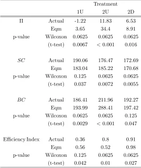
Our first evidence is on aggregate auction outcomes. For each auction in the data, we record the actual outcome on key variables (efficiency, supplier profits, and total production and procurement costs). Then we compute predicted outcomes that would have occurred (for this cost triple), if the subjects had played the strategies derived in Section 3.19 Then we average these actual and predicted outcome variables across all auctions within a session to form a session mean. If our subjects play mutual best responses to each other, then these actual and predicted session means should be close. We test this by comparing (for each treatment) the five matched pairs of session means, using both a non-parametric Wilcoxon signed rank test and a paired t-test.20
The values are in francs per auction; to convert to dollars per session, multiply by 0.6 (30 auctions/session·$0.02/franc). Note that the statistical tests are conservative – by taking session means as the data points, we do not make any assumptions about the independence of outcomes within a session – but as a result they have relatively low power. In particular, for the Wilcoxon test with n = 5, the strongest possible rejection of no difference between actual and predicted outcomes is a p-value of 0.0625; we will refer to this as a significant difference, and to the next smallest p-value (0.125) as marginally significant.
In all three auction formats, subjects earn significantly lower profits than would be predicted by equilibrium; the difference, in dollars per subject per session is $2.92 for 1U, $13.54 for 2U, and $1.43 for 2D. In percentage terms, subjects earn 34% of their equilibrium profits in 2U and 73% in 2D. In 1U, subjects earn -33% of their equilibrium profits since they actually lose money on average. Profits per auction are the residual between the total production cost of the three units sold (SC, for supplier cost) and the total revenue from selling those units (BC, for buyer cost). The shortfall of actual profits can be attributed partly to stronger than expected competition –
BC is significantly lower than predicted in all three formats (marginally so for 2D). The other factor to blame for low profits in 1U and 2D is inefficient production – SC is higher for both treatments (significantly for 2D, marginally significant for 1U) than in equilibrium. The last row normalizes suppliers’ production cost into an index ranging from 0 (costs were no better than a random allocation) up to 1 (the allocation was efficient).21 The comparison of actual to equilibrium values of this index is similar to those for SC. Note that in the case of 2U, the fact that subjects
19
For 1U, where the equilibrium strategies for some types are mixed, we compute the expectation of the outcome variable, for each auction.
20
Note that session means could be close even ifindividual auctions do not conform closely to the predictions. In
this sense, a rejection of equality in our tests is a strong refutation of the predictions. However, we will interpret the results cautiously because the predictions are based on strategies that are approximate joint best responses for the discrete cost type case.
21
More precisely, the index isEf f iciency Index= SCrand−SCg
SCrand−SCef f, where gSC is either the actual supplier cost, or
do not play the pooling equilibrium strategies means that allocations are more sorted by cost (and so, more efficient) than predicted.
Treatment
1U 2U 2D
Π Actual -1.22 11.83 6.53
Eqm 3.65 34.4 8.91
p-value Wilcoxon 0.0625 0.0625 0.0625
(t-test) 0.0067 < 0.001 0.016
SC Actual 190.06 176.47 172.69
Eqm 183.04 185.22 170.68
p-value Wilcoxon 0.125 0.0625 0.0625
(t-test) 0.037 0.0072 0.0055
BC Actual 186.41 211.96 192.27
Eqm 193.99 288.41 197.42
p-value Wilcoxon 0.0625 0.0625 0.125
(t-test) 0.0029 < 0.001 0.047
Efficiency Index Actual 0.36 0.8 0.91
Eqm 0.56 0.52 0.98
p-value Wilcoxon 0.125 0.0625 0.0625
[image:16.612.161.450.115.461.2](t-test) 0.042 0.01 0.027
Table 3: Actual Behavior versus Equilibrium Predictions (francs per auction) Π is the (avg.) Profit per supplier, SC the (avg.) total cost of the suppliers selected to produce, BC the (avg.) total cost of the buyer, and Efficiency = 1 if the efficient suppliers were selected.
Table 3 suggests that for auction format 2D, equilibrium predicts actual session level outcomes reasonably well. Although there are statistically significant gaps between actual and predicted outcomes, those gaps are small in magnitude. In the other two treatments, the gaps between equilibrium predictions and actual outcomes are substantially wider. It is conceivable that these gaps could narrow in later rounds as subjects gain experience with the auction format. To check for this, we computed the profit shortfall (predicted minus actual profits) for rounds 1-15 and 16-30 of each session, normalized to dollars per 15 rounds. For auction format 2D, the average (across sessions) shortfall does decline over time, from $0.85 to $0.58. (The sum of these is the $1.43 reported earlier.) However, in the other two auction formats there is little change: in 1U the shortfall declines from $1.49 to $1.43, while in 2U it rises from $6.69 to $6.82.22 Thus the condition
22
that subjects play mutual best responses appears to fail persistently in some of our settings. Figure 2 breaks down the actual and equilibrium predicted subject payoffs by cost type.23 Remember that in our setting, an efficient allocation usually requires the smallest and largest realized suppliers to produce one and two units respectively. The median realized type is what VBW (1996) call a “marginal efficient seller” at both scales of production: he is second-best at producing both quantities that are needed and should sit out. VBW argue that in their setting, these marginal sellers compete too vigorously, lose money on average (due to exposure problems), and contribute to volatile market outcomes. In our setting, it is the flexible cost types who are most likely to be the marginal seller. In 1U (where exposure problems are most severe) these types indeed lose money on average, suggesting that they may contribute to volatile outcomes by bidding too aggressively. However, large bidders also lose money in 1U, and the profit shortfall (of actual profits relative to equilibrium predictions) is shared across all cost types in 1U and 2U. In contrast, in 2D, suppliers with declining average costs (the large and flexible types) earn average payoffs quite close to the predicted ones.
However, Figure 2 cannot tell us whether, for example, large suppliers in 1U appear to do poorly because of their own errors, or because their profit opportunities are limited by other bidders’ mistakes. (For example, if small suppliers bid too aggressively, then prices fall and the inframarginal profits that large suppliers rely on dry up.) In the remainder of the paper, we try to separate these issues by focusing on whether subjects play best responses to the empirical opponent bidding that they actually faced.
4.2 Actual vs. Best Response Bidding
In this section, we construct the payoffs that a subject could have earned by best responding to the distribution of her opponents’ past play; then we ask how subjects’ actual payoffs compare to these computed best response payoffs. This can provide a clearer test of how effectively subjects optimize than the benchmark profits in Table 3 do, since the latter may have been simply impossible to achieve given opponents’ actual bidding.
The rationale for computing best responses with respect topast play is that it would be both feasible and reasonable for a subject to base her expectations about her current opponents’ bidding on her own past market experience. There are two caveats to this approach. One is our im-plicit assumption that subjects can draw reasonably accurate inferences about past opponent bids from market feedback. Thus success in best responding may partly reflect the richness of market feedback, and subjects’ success in interpreting it. The second caveat is that in a volatile market
significance (p-value 0.125) in a Wilcoxon test over the five session means. We also tested the difference
Shortf all1−15−Shortf all16−30 for the five sessions of each treatment to determine whether there is a significant
improvement in the gap between actual and predicted profits. There is no significant improvement (for any treatment).
23
environment, a best response to past play might not be a particularly good strategy in the current round. Later in this section, we will show that subjects would have systematically improved their payoffs if they had always chosen best responses to past play. Thus, using these best responses as a benchmark for subjects’ behavior seems reasonable.
When an arbitrary bidbis referred to in what follows, it should be interpreted as either a scalar or a pair, depending on the treatment. Define πit(b) to be the payoff that i would have earned
by playing b under her round t costs, against her opponents’ round t bids. Let bit be the bid she
actually used, andπit =πit(bit) the payoff she actually earned.
Next we construct the predicted payoff given past play, Hit(b), defined as the expected payoff
that i would earn by playing b in round t, under her round t costs, against the distribution of opponent bids that she faced in rounds 1 to t−1. To do this, first define πt
iτ(b) to be the payoff
that i would have earned by playing b against her round τ opponents, under her round t costs. Then Hit(b) is defined as:
Hit(b) =
1
t−1
t−1
X
τ=1
πiτt (b) .
We say that a subject best responds to past play if she chooses a bid in round t that max-imizes Hit(b). We define ¯Hit to be the payoff that she would actually earn in round t by best
responding:24,25, 26
¯
Hit≡πit(b∗) whereb∗ = arg max b∈B Hit(b)
We start by asking how actual profits compare to what subjects could have earned by best responding to past play. We determine how much more money a subject could have earned over 30 rounds by best responding to past play, relative to subjects’ actual earnings. The average value of
¯
Hit−πit for each treatment, converted to dollars per 30 rounds, is $1.64 for 1U, $3.03 for 2U, and
$0.52 for 2D.27 Thus, subjects leave less money on the table than the comparison to equilibrium
payoffs in Table 3 would suggest. For 2D, these foregone profits are a relatively small fraction (14%) of the average 30 round profit of $3.84. However, the foregone profits represent 42% of average actual profits in 2U ($7.25), while in 1U the foregone profits would have saved subjects from losing money on average (-$0.52).28 Furthermore, these foregone profits persist; over the last 15 rounds they average $1.65 (1U), $2.85 (2U), and $0.42 (2D) respectively (still measured in $/30 rounds).
24
IfHit(b) has more than one maximizer – sayb∗1,b ∗
2, ... – then we average overπit(b∗1),πit(b∗2), ... to get ¯Hit.
25
As a secondary benchmark, we also computed a ‘full information’ best response. F Iit(b) is the expected payoff
that b would earn (under round t costs) against the distribution of opponent bids that i faces in all 30 rounds. Similarly,F Iit is the round tpayoff thatiwould have actually earned by choosing a maximizer of F Iit(b). When
past and future opponent bidding differ substantially, profitsF Iit and ¯Hit will tend to differ; to achieve profitF Iit,
a subject would need to be good at forecasting opponents’ future bids. In our data,F Iit tends to be higher than ¯Hit,
while actual payoffs generally fall short of ¯Hit. Given this, our analysis focuses on the less demanding benchmark.
26
Of course, there is no guarantee that ¯Hit will be the largest possible profit for choiceit, since it is determined on
the basis of opponents’ past, not current play.
27
In each case, we average ¯Hit−πitover all choice situationsit, then multiply by
3
5 = (30 rounds) / (50 francs/$). 28
However, the average foregone profit over an entire treatment does not provide a full picture of how closely actual profits match up with ¯Hit on a round by round basis. To assess this, we next
calculate the mean of the squared deviation ¯Hit−πit 2
. This value (in francs per choice situation) is 322 for 1U, 540 for 2U, and 61 for 2D.29Thus, auction by auction, actual profits πit track ¯Hit
reasonably well in 2D, but less well in 1U and 2U.
Altogether, this preliminary analysis suggests that best responding to opponents’ past play is a plausible model of actual behavior in treatment 2D, but does not describe actual behavior in 1U and 2U as well. In the remainder of the paper, we explore these deviations from best response behavior, argue that they can be attributed to imperfections in profit maximization, and assess explanations that could explain these imperfections. We favor explanations that can fit into a general model of bidding across all three treatments, rather than explanations that would require fundamentally different behavior in different treatments. Loosely, one might categorize these explanations according to whether they relax the “profit” or the “maximization” side of the standard model of behavior. That is, one class of explanations (alternative preferences) would be that subjects are successful maximizers, but that their utility functions include objectives other than profits (reducing risk or losses, for example). Another class of explanation (hard maximization) is that subjects do care about profits, but their profit maximization problem is challenging, and its “degree of difficulty” varies across auction formats. We find only mixed support for the first class of explanation and considerable support for the second. We will argue that theways in which subjects stumble when confronted with challenging maximization problems are both systematic and instructive, and hence should be considered when evaluating the tenableness of equilibrium predictions.
5
Bidding Based on Modified Best Responses: Model
In this section, we construct and estimate a model of bidding in the spirit of Erev and Roth’s (1998) reinforcement learning and Camerer and Ho’s (1999) experience weighted attraction (EWA) learning. Our first objective is to study whether an explanation based on preferences, or one based on noisy optimization, better explains deviations from best response behavior. One criterion of a successful model will be its generality: that is, how well it can explain bidding under all three auction formats.
Suppose that subjecti’s probability of choosing bidbin roundtdepends on a propensityPit(b)
according to a standard logistic formulation:
Pr (bit=b) =
ePit(b)
P
˜
b∈Be Pit(˜b)
, t∈ {2,3, ...,30} (1)
for the corresponding session of 2D). For both 1U and 2U, Session 1 is the anomaly: ¯Hit−πit is negative (subjects
do better than the best response profit, and by a larger margin than for 2D). We will offer a partial explanation for this anomaly later.
29
where B is the strategy space. (Subjects’ initial bids in round t = 0 are left unmodeled.) The propensity is assumed to depend on a linear combination of influences includingHit(b) and possibly
other factors:
Pit(b) =βHit(b) + [other terms] . (2)
As a baseline, we start with what we will call thePure Profit (PP) model.
ModelPP: Pit(b) =βHit(b) (3)
The previous section presented indirect evidence about whether subjects choose a maximizer of
Hit(b). Model PP broadens the question to ask how emphatically subjects favor bids with higher
profits over bids with lower profits.30 We begin by testing the hypothesis that a single coefficient
β can explain how subjects respond to profits across all three treatments. To do this, we estimate model PP by maximum likelihood separately for each session of each treatment.31 This generates fifteen (independent) estimates ofβ. Table 4 presents the five estimates ofβfor each treatment, and their mean.32 These five estimates are compared for each pair of treatments with both Wilcoxon signed rank tests and t-tests. While subjects respond more strongly to profits in 2U than in 1U, the difference is not significant. However, subjects do respond to profits much more vigorously in 2D than in the other two treatments, and these differences are highly significant.
Price feedback may partially explain this gap. In treatment 2D, prices reveal all of the winning bids, and this may make it easier for a subject to determine how competitively she must bid in order to win. In the other treatments, the winning inframarginal bid is not revealed by the price; this may contribute to the difficulty that subjects have in identifying profit opportunities.
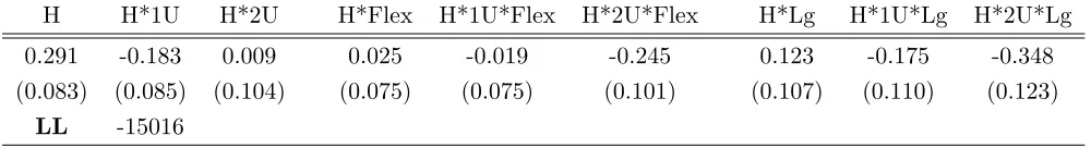
Next we ask whether the difference between 2D and the other two treatments depends on the supplier’s cost type or how experienced she is. We estimate model PP on the pooled data (all 15 sessions) interacting Hit(b) with treatment dummies for 1U and 2U (with 2D omitted). We
also include interactions with treatment and cost type (flexible or large, with small omitted), or with treatment and roundt. The coefficients are presented in Table 5. Small suppliers are equally
30
Note that this model,viathe definition ofHit(b), puts equal weight on a subject’s experience in all past rounds
1 through t−1. One might expect that because costs change every six rounds subjects would put greater weight on their most recent experience. (Many learning models, such as Camerer and Ho’s EWA learning model, build in a ‘decay’ factor that can capture this type of effect.) However, when we tested models with a decay factor, we found that the equal-weighting model actually performs better in our data.
31
For each of these fifteen estimations, each decision opportunity for a subject in rounds 2 through 30 is treated as a single observation. To sidestep computational difficulties related to the size of the strategy space for 2U and 2D, we followed McFadden’s procedure (McFadden 1978, Train et al. 1987) of generating consistent estimates by sampling the strategy space. (Further details are in the appendix.)
32
Session p-value on test of equality against:
Mean 1 2 3 4 5 1U 2U 2D
1U 0.110 0.175 0.084 0.051 0.132 0.106 signrank - 0.625 0.0625
t-test - 0.392 0.006
2U 0.160 0.389 0.213 0.067 0.058 0.075 signrank - 0.004
t-test - 0.0625
[image:21.612.87.528.75.191.2]2D 0.391 0.496 0.557 0.261 0.316 0.325
Table 4: Session by session coefficients onHit(b) for model PP
H H*1U H*2U H*Flex H*1U*Flex H*2U*Flex H*Lg H*1U*Lg H*2U*Lg
0.291 -0.183 0.009 0.025 -0.019 -0.245 0.123 -0.175 -0.348
(0.083) (0.085) (0.104) (0.075) (0.075) (0.101) (0.107) (0.110) (0.123)
LL -15016
Table 5: Model PP estimated on pooled data, with treatment and cost type interactions (Baseline is treatment 2D). Standard errors are clustered by the 15 sessions.
responsive to profits in 2D and 2U. (In 1U they do worse.) As avoidable fixed costs get larger (the flexible and large interactions), the treatments diverge: profit responsiveness improves in 2D and deteriorates in the other two treatments.
One might wonder whether this performance gap is transient – perhaps subjects just need a few more rounds to sort out best responding in 1U and 2U than they need in 2D. The regression with round interactions refutes this fairly emphatically (Table 6). Responsiveness to profits not only starts at a higher level in 2D, but it also rises far faster with experience in 2D. While the coefficient onHit(b) does rise over time in the other two treatments (at a rate given by the sum of
theH∗tand H∗t∗1U orH∗t∗2U coefficients), but the improvement is anemic.
[image:21.612.71.571.238.306.2]H H*1U H*2U H*t H*t*1U H*t*2U
0.163 -0.091 -0.112 0.016 -0.015 -0.014 (0.031) (0.036) (0.033) (0.003) (0.003) (0.003)
LL -15026
Table 6: Model PP estimated on treatment and round interactions (Baseline is treatment 2D). Standard errors are clustered by the 15 sessions.
5.1 Payoff Volatility
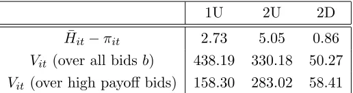
Earlier, we suggested that avoidable fixed costs and auction rules can interact to produce a volatile environment for bidders; now we introduce measures of that volatility, Vit(b), which is a natural
counterpart to Hit(b). While Hit(b) measures the average of a sequence of hypothetical payoffs n
πt
i1, πit2, ..., πi,tt −1
o
thatbwould have earned against past opponents,Vit(b) measures thevariance
of that sequence. Formally, define:33
Vit(b) =
1
t−1
t−1
X
τ=1
πiτt (b)−Hit(b) 2
(4)
Table 7 presents mean values ofVit(b) across the three treatments. Each mean is taken over all
possible bids b ({0, ...,100} or{0, ...,100}2) for every choice situationit. The substantially higher values of Vit(b) in treatments 1U and 2U (relative to 2D) indicate that in the two uniform price
treatments, a typical bid’s hypothetical performance in past rounds tends to vary a lot depending on which past round is considered. By averagingVit(b) over all possible bids, the summary statistics
in Table 7 include weight on the payoff variability of some truly abysmal bids that subjects are unlikely to seriously consider. In the next line of Table 7, we take the average of Vit(b), but this
time include only those bids in the top decile of Hit(b), for each choice situation it. When we
consider the variability of only these ‘high payoff’ bids, 2U looks more volatile than 1U, but both are still more volatile than 2D.34
Based on these summary statistics, it seems plausible that payoff volatility as measured by
Vit(b) could help to explain deviations from best response behavior in 1U and 2U. We propose two
main channels through whichVit(b) might affect bidding. The first is based onpreferences. Suppose
that subjects are risk averse and able to estimate both Hit(b) and Vit(b) reasonably well. When
choosing bids, they will tend to penalize riskier ones (highVit(b)); then in riskier environments like
1U and 2U, actual bids may diverge relatively more from risk neutral best responses.
Associated with this preference-based argument for deviations from best response behavior,
33
Of course, the statistically correct sample estimate of payoff variance would normalize by 1
t−2, not 1
t−1. This
would require us to give up the first two rounds of data in the estimation (instead of just the first round). Rather than do this, we use the formula as stated, and accept the implicit restriction thatVi2(b) = 0 for allb. This has no
material effect on the results.
34
Session by session comparisons ofVit in 1U vs. 2D or 2U vs. 2D both reject equality (Wilcoxonp-value 0.0625),
1U 2U 2D ¯
Hit−πit 2.73 5.05 0.86
Vit (over all bids b) 438.19 330.18 50.27
[image:23.612.178.436.72.140.2]Vit (over high payoff bids) 158.30 283.02 58.41
Table 7: Summary Statistics forVit(b)
we propose the The Risky Payoff (RP) model. Under the RP model, we conjecture that subjects dislike risk and bid with the aim of maximizing the simple mean-variance objective functionHit(b)−
rVit(b), where r≥0. 35
ModelRP: Pit(b) =β(Hit(b)−rVit(b)) (5)
The second channel through which Vit(b) might affect bidding is based on noisy optimization.
Define the empirical standard deviation of a bidσit(b) = p
Vit(b). Suppose that subjects are risk
neutral, but their attempts to estimate expected payoffs Hit(b) are confounded by the fact that
these payoffs are volatile. We suggest two versions of this noisy optimization story; they have similar empirical implications and we will not try to distinguish them in the data. One version is that when a bid’s returns have been volatile (σit(b) large), a subject makes larger errors in estimating
Hit(b). The other is that a subject is able to estimate Hit(b) accurately, but like a statistician,
places less confidence on this estimate if σit(b) is large. In the first case, a subject may respond
strongly to the profit that she perceives, but because this perception is inaccurate, we will measure this as a weaker response to Hit(b). In the second case, it is the subject herself who dials down
her response because she suspects that the magnitude ofHit(b) (either positive or negative) may
be large simply by chance.
Associated with this imperfect/noisy optimization-based argument for deviations from best response behavior, we propose the Noisy Payoff (NP) model. Under the NP model, we assume that subjects are less sensitive to expected payoffs for bids that are noisy:
ModelNP: Pit(b) = (β−γσit(b))Hit(b) (6)
Note that while both models RP and NP rely on payoff variability, they do so in (testably) different ways: in RP,Vit(b) enters directly, whereas in NP, it enters only through the interaction
Hit(b)σit(b).36 Furthermore, RP predicts that high payoff variability always makes a bid less
attractive, while NP predicts that noise disguises how bad some bids (those withHit(b)<0) are,
making them more likely to be chosen.
35
In earlier versions of the paper that did not include a learning model, we computed best responses under CARA and CRRA utility and found qualitatively similar patterns across treatments to those that we will report for model RP. Here, with the mean-variance formulation, we err on the side of simplicity.
36
We useσit(b) in model NP rather thanVit(b) partly because of the analogy to confidence interval analysis, and
partly because it fits the data better. However, comparisons between models RP and NP do not change if we use
5.2 Bids below cost: loss aversion and weak dominance
As subjects consider the bidding landscape, bids below cost play an interesting role. In two of our auction formats, 1U and 2U, profit maximization may sometimes require placing a bid below cost, which in principle could lose money for some realizations of the opponents’ bids (This is not true in 2D, where optimal bids are always above cost.). However, not all bids below cost are potentially profitable. There are also some bids below cost that are dominated and could never be optimal.
There is considerable evidence that people do not treat gains and losses symmetrically (Kah-neman et al. (1991)), as manifested in a number of types of behavior which collectively have been termed “loss aversion.” If subjects have preferences that penalize loss exposed bids, this could help to explain why profit maximization is apparently weaker in 1U and 2U. It is also possible that some subjects will avoid dominated bids – perhaps because it is particularly salient that they are unprofitable – without avoiding other loss exposed bids.37 In this case, the behavior suggests not
loss averse preferences but rather that dominance helps subjects to optimize more accurately. Define a bid as loss exposed, with indicator variable Lit(b), if there is some set of opponent
bids for which it could conceivably return a negative payoff. The values ofLit(b) are summarized
in Table 8. Table 8 also presents a summary of the bids that subjects actually chose: Note that choosing a loss exposed bid is very common in 1U and rarer in 2U. These summary statistics hint that it may be difficult for loss aversion to simultaneously explain bidding in both 1U and 2U.
Associated with this preference-based argument for deviations from best response behavior, we propose theThe Loss Exposed (L) model which includes an indicator for loss exposed bids. Under the L model, we conjecture that subjects would avoid submitting bids that are loss exposed if they have loss averse preferences.
ModelL: Pit(b) =βHit(b) +γLLit(b) (7)
We define another indicator variable Domit(b) equal to 1 if bid b is weakly dominated. The
values ofDomit(b) are summarized in Table 8 in each case, the weakly dominated bids are a subset
of the loss exposed ones. Note that choosing a dominated bid is rare in all three treatments, while, as noted above, choosing a loss exposed bid is very common in 1U and rarer in 2U. These combined summary statistics hint that the avoidance of bids below cost may be better explained as a result of (possibly imperfect) profit maximization calculation.
Associated with this imperfect optimization-based argument for deviations from best response behavior, we propose theThe Dominated Bids (Dom)model which includes an indicator for weakly dominated bids. Under theDom model, we conjecture that subjects would avoid submitting bids that are weakly dominated (but would not avoid bids below cost that are undominated).
ModelDom: Pit(b) =βHit(b) +γDomDomit(b) (8)
37
1U 2U 2D
Lit(b) = 1 iff. b <max(c1, c2) b1 < c1 orb2 < c2 b1 < c1 orb2< c2
Domit(b) = 1 iff.
forc1 ≤c2 b < c1 max(b1, b2)≤c2 “
forc1 > c2 b <2c2−c1 max(b1, b2)≤c1 “ #(chosen bid was loss exposed)
#( choice situations) 0.721 0.149 0.015
#(chosen bid was dominated)
[image:25.612.103.509.73.193.2]#( choice situations) 0.105 0.079 0.015
Table 8: Dominated and loss exposed strategies
5.3 Payoff landscape
Another factor that could make optimization difficult for subjects is the shape of the profit land-scape. (In this case, there is no alternative based on preferences to compare to directly.) To fix ideas, if Hit(b) is strictly quasiconcave in b, we will consider this an easy optimization problem.
Concisely characterizing the features of a landscape that make optimization difficult is itself a no-toriously difficult problem.38 We focus on a definition that, while somewhat ad hoc, is intuitive
and simple. For a choice situationitand a bidb, we say that b is a local maximum if its expected payoffHit(b) is weakly greater than that of every neighboring bid. (For the one dimensional bids
in 1U, neighboring bids are b−1 andb+ 1. In the other two treatments, we take the four nearest neighbors tob= (b1, b2); that is, (b1±1, b2) and (b1, b2±1).) For choice situationit, defineLMit
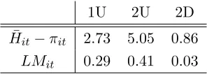
to be the fraction of bids (over the strategy space B) that are local maxima.
We conjecture that subjects will appear less sensitive to expected profits in choice situations in whichLMit is large. This could occur if subjects search locally for payoff-improving strategies;
in this case, they will tend to get stuck at local maxima. Alternatively, subjects may try to take a global view of Hit but find it hard to discern patterns in the landscape. Mean values of LMit
(see Table 9) indicate that subjects in 1U and 2U tend to face payoff landscapes with many local maxima, suggesting thatLMit may help to explain the disparity in best response behavior across
treatments.
1U 2U 2D
¯
Hit−πit 2.73 5.05 0.86
LMit 0.29 0.41 0.03
Table 9: Values of LMit across treatments
Associated with this imperfect optimization-based argument for deviations from best response behavior, we propose theThe Local Maximum (LM) model. As n model NP, we introduceLMitas
38
[image:25.612.232.380.550.603.2]