A deterministic tabu search algorithm for the capacitated arc routing problem

(1)

www.elsevier.com/locate/cor

A deterministic tabu search algorithm for the capacitated

arc routing problem

José Brandão

a,∗

, Richard Eglese

b

a_{Dep. de Gestão, Escola de Economia e Gestão, Universidade do Minho, Largo do Paço, 4704 -553 Braga, Portugal} b_{Department of Management Science, Lancaster University Management School, Lancaster LA1 4YX, UK}

Available online 25 September 2006

Abstract

The capacitated arc routing problem (CARP) is a difﬁcult optimisation problem in vehicle routing with applications where a service must be provided by a set of vehicles on speciﬁed roads. A heuristic algorithm based on tabu search is proposed and tested on various sets of benchmark instances. The computational results show that the proposed algorithm produces high quality results within a reasonable computing time. Some new best solutions are reported for a set of test problems used in the literature.

Keywords:Heuristics; Arc routing; Tabu search

1. Introduction

The capacitated arc routing problem (CARP) may be described as follows: consider an undirected connected graph

G=(V , E), with a vertex setVand edge setEand a set of required edgesR⊆E. A ﬂeet of identical vehicles, each of capacityQ, is based at a designated depot vertex. Each edge of the graph(vi, vj)incurs a costcij whenever a vehicle

travels over it or services a required edge. When a vehicle travels over an edge without servicing it, this is referred to as deadheading. Each required edge of the graph(vi, vj)has a demandqijassociated with it. A vehicle route must start

and ﬁnish at the designated depot vertex and the total demand serviced on the route must not exceed the capacity of the vehicle,Q. The objective of the CARP is to ﬁnd a minimum cost set of vehicle routes where each required edge is serviced on one of the routes.

In the instances tested, the objective is to minimise the total cost incurred on the routes and does not include any costs relating to the number of routes or vehicles required.

The graph or network on which the problem is based may be directed or undirected or mixed, but in this paper only undirected graphs are considered. A good introduction to and survey of the CARP and other arc routing problems may be found in Dror[1].

In the CARP, each edge in the graph may model a road that can be travelled in either direction and each vertex corresponds to a road junction. Applications of the CARP arise in operations such as postal deliveries, household

∗_{Corresponding author.}

(2)

waste collection, winter gritting, snow clearance and others, though in most practical applications there are additional constraints that must also be considered, including time window constraints or restrictions on certain turns (see e.g. Lacomme et al.[2]).

The CARP is NP-hard. Even when a single vehicle is able to service all the required edges, the problem reduces to the rural postman problem (RPP) which has been shown to be NP-hard by Lenstra and Rinnooy Kan[3]. Additionally, Golden and Wong[4]showed that even 1.5-approximation for the CARP is NP-hard. Exact methods for the CARP have only been able to solve relatively small examples to optimality.

A discussion of different heuristic algorithms that have been proposed for the CARP can be found in Dror[1]. These include simple constructive heuristics (e.g. Pearn[5,6]) and go on to include various metaheuristic algorithms. The most successful algorithms that have been reported in the literature are based on different metaheuristic models. We have chosen two of these with which to compare the results of our proposed algorithm. The ﬁrst is the tabu search based algorithm known as “CARPET” which is described in Hertz et al.[7]. The second is the approach using memetic algorithms, which will be referred to as MA, described in Lacomme et al.[8].

Beullens et al.[9]describe a guided local search heuristic for the CARP and also introduce some new large data sets based on the inter-city road network in Flanders (Belgium). Our proposed algorithm is also tested on these data sets.

There are also other notable contributions that have recently been proposed for solving the CARP. Greistorfer[10]

also uses a tabu search based approach, but uses a form of scatter search within his proposed heuristic. Hertz and Mittaz

[11]describe a variable neighbourhood descent algorithm for the CARP. Amberg et al.[12]have also proposed a tabu search based algorithm; their approach makes use of capacitated trees and can be applied to multi-depot problems. Baldacci and Maniezzo[13]describe an exact method for solving the CARP based on a new transformation to a constrained node routing problem. A similar approach is described by Longo et al.[14]who also obtain bounds and solutions to standard test problems using a transformation to the constrained vehicle routing problem.

The approach described in this paper is based on a tabu search algorithm (TSA). However, it differs from CARPET in many of the details of the implementation. In particular, the algorithm presented here is deterministic and does not require the use of random parameter values (which are also needed for MA), so making the results fully reproducible. The structure of the remainder of this paper is as follows. Section 2 describes the methods used to obtain initial feasible solutions in our algorithm. Section 3 describes the TSA for solving the CARP and Section 4 describes the results obtained on a set of test problems. Final conclusions are presented in Section 5.

2. Initial solutions

Five different methods were used to obtain initial solutions. Each method provided a feasible solution that could be used as an initial solution for the TSA. The methods were designed to be fast to compute and to provide a variety of starting solutions for the TSA to improve. The diversity provided by the different starting solutions was found to be useful in ultimately ﬁnding high quality solutions.

When implementing the algorithms described in this paper, each route was represented by an ordered list of vertices, starting and ending with the depot vertex, together with a corresponding ordered list of zero–one variables,type_p. If the pth vertex in the list isvi and it is immediately followed byvj, thentypeptakes the value one if(vi, vj)is a required

edge which is serviced at this stage of the route. The cost of the route includescij and the demand satisﬁed by the

vehicle on this route includesqij. If(vi, vj)is not a required edge which is serviced at this stage of the route, thentypep

takes the value zero,(vi, vj)represents a path and the cost of the route is increased by the cost of deadheading this

path, which is the shortest path fromvi tovj. This representation allows all the required operations and calculations to

be carried out efﬁciently.

2.1. Method 1—cheapest edge

(3)

included edge (and which has least cost in the event of ties, with ties broken arbitrarily if more than one edge has the same least cost), but excluding any edge that closes the tour unless no others are feasible in terms of vehicle capacity. If the next required edge is not incident to the last vertex on the route so far, the cost of the route includes the cost of deadheading along the least cost path between the last vertex and the next edge. When no remaining required edges can be feasibly added to a route, the route is completed by the vehicle returning to the depot along the least cost path from the end of the last serviced edge, and the next route is started.

2.2. Method 2—dearest edge

This method operates in exactly the same way as Method 1, except that the highest cost edge replaces the lowest cost edge at each selection point.

2.3. Method 3—insert

Each route is started as in Method 1 and a route is completed by adding the deadheading path from the end of the ﬁrst edge back to the depot. Then the next edge to be chosen from the required edges not yet served and which is feasible in terms of vehicle capacity is the one that increases the cost of the route by the least amount. When considering an edge for insertion, the new edge may be inserted between any pair of required edges already included in the route that are currently linked by a deadheading path, or before the ﬁrst edge or after the last edge if these edges are not directly linked to the depot.

2.4. Method 4—connected components

This method requires the use of a procedure to solve the RPP for sets of connected required edges. The RPP is the problem of finding the minimum cost single route to service a set of required edges in an undirected graph and in general is NP-hard[3]. However, when the subgraph generated by the subset of required edges is connected, the RPP is reduced to the undirected Chinese postman problem which is polynomially solvable[15]. A general heuristic for the RPP was first proposed in Frederickson[16], based on a procedure that is similar to Christofides’ heuristic for the undirected travelling salesman problem[17]. The method has been described and used by several researchers; our version follows the version described in Pearn and Wu[18](though in that paper it is referred to as “Christofides et al. algorithm”).

Frederickson’s algorithm is described in general here as it is also used within the TSA to improve individual routes. In what follows, ER =R for this initial solution method. However, when this algorithm is used to improve

routes individually in the TSA, thenER ⊆ R includes only those required edges serviced by that particular route.

Frederickson’s algorithm may be described as follows:

1. LetGR=(VR, ER)be the subgraph of Ggenerated byER with the corresponding set of verticesVR. LetCi

(i=1, . . . , c)be theith componentGR. LetGCbe the graph derived fromGby reducing each componentCiofGR

to a single vertex inG. The cost of an edge(i, j )∈GCis deﬁned as d(i, j )=d(Ci, Cj)=minx,y{d(x, y)−ux−uy},

wherex, y∈V,x∈C1,y∈C2andux= −(deg(x)−2). d(x, y)is the cost of the minimum cost path fromxto

yin the original graphGand deg(x)is the degree of vertexxin the original graphG.

2. Determine the minimum cost spanning tree inGC. LetETbe the set of edges from the minimum cost spanning

tree solution.

3. Considering the graphGR∪ETﬁnd a minimum cost perfect matching of the odd degree vertices. LetEMbe the

edges of the matching.

4. Find an Eulerian tour in the graphGR∪ET∪EM. This tour is the RPP solution.

Pearn and Wu show how the results can be inﬂuenced by the use of a parameter. In our implementation, the algorithm is executed with=0, then=1 and the better solution is chosen.

(4)

complex algorithm was not available and so a simple greedy heuristic was used for the matching step, which can be described as follows:

Step0: Set every vertex as non-included.

Step1: Select the edge with the minimum cost among all the edges of the graph, linking two non-included vertices. Set the two end vertices of this edge as included.

Step2: Repeat step 1 until all the vertices are included.

If the number of vertices were less than or equal to six, then the heuristic was not applied and the optimum solution was found by complete enumeration. Tests were carried out to see what effect the use of this procedure had on the solution to the CARP by ﬁnding the optimum solution to the matching problem by complete enumeration in all cases. As expected, the complete enumeration method was much slower than the procedure using the heuristic, but surprisingly, the average solutions to the CARP were worse than when the heuristic was used. We therefore retained the heuristic procedure for solving the matching problem.

Thus for each connected component, a route is constructed using Frederickson’s heuristic, ignoring the capacity constraints. In the special case where more than two required edges are adjacent to the depot vertex, the connected component is split again into connected components in which no more than two required edges connect to the depot. This is done by splitting the route into subroutes: following the order of the route it is cut at the point where the second edge linked to the depot appears; then a new route starts and this process ﬁnishes when only one or two edges linked to the depot remain.

The route is modified into one starting and ending at the depot by starting with a required edge connected to the depot if one exists, otherwise adding the least cost route from the depot to a required edge in the connected component, following the constructed route until the last required edge in the connected component has been included and then finally joining the route to the depot by linking back to the depot along the least cost path. If any route is infeasible according to the capacity constraint, it is split into smaller routes in the following way. Starting from the depot, the route is followed until the last feasible required edge has been included. The route is then completed by adding the least cost path from the end of this edge back to the depot. The next route is started by adding the least cost path from the depot to the next required edge that is to be served on the route that had been created. The process finishes when all required edges in each connected component have been included in a route.

2.5. Method 5—path scanning

This method is based on the procedure proposed by Golden et al.[19]. Each route is extended by one required edge at each step using a variety of selection rules.

Each route starts at the depot vertex. LetSbe the set of required edges closest to the end of the current route that are not yet served and do not exceed the capacity of the current route. IfSis empty then complete the current route using the shortest deadheading path from the end of the current route to the depot vertex and start a new route. IfSis not empty, exclude fromSany edges that would close the route unless that would makeSempty. Select a required edge in Sto be the next edge in the route to be serviced according to the current rule and extend the current route to the vertex at the end of the selected edge.

Five rules are used to determine the next required edge,e, in the route to be serviced: (1) maximise the distance to the depot; (2) minimise the distance to the depot; (3) use rule 1 if the vehicle is less than half-full, else use rule 2; (4) maximise the ratiod(e)/c(e), whered(e)andc(e)are, respectively, the demand and the cost ofe; (5) minimise this ratio. Each criterion gives rise to one solution and the best of the ﬁve is chosen.

Some results to show the effectiveness of these initial solution methods are given in Section 4.

3. The tabu search algorithm

3.1. Neighbourhood moves

The TSA is based on three types of neighbourhood move. The ﬁrst two are insertions (single and double) and the third is a swap.

(5)

linked by a deadheading path of edges. The trial insertion considers both directions for the edge to be traversed when inserted in the new route. In a double insertion move, the operation is similar except that a candidate consists of two connected required edges in one route.

The swap move is similar. Two candidate edges are selected from two different routes, each containing deadheading paths. The candidate edges are removed from their original routes and inserted in the other routes between any two serviced edges that are not adjacent, but are linked by a deadheading path of edges.

In this implementation, the frequencies of the different types of move may change according to the phase of the algorithm. Parameters,FSI,FDIandFSWAPdenote the frequencies of the single insertion, double insertion and swap

moves, respectively. For example, the value ofFSWAPimplies that the swap move is only tested everyFSWAPiterations.

The trial move chosen depends on the effect of the move on the objective function deﬁned in the next section.

3.2. Objective function

The objective function to be minimised by the TSA includes the total cost of each route,i, plus a penalty costP w(i), wherePis a penalty term andw(i)=max(x(i)−Q,0), and wherex(i)is the sum of the demands on the edges serviced in routei. For any candidate solution,S, the objective function is denoted byf (S).

The parameterPis set at 1 initially, and is then halved if all the solutions are feasible for 10 consecutive iterations; it is doubled if all the solutions are infeasible for 10 consecutive iterations. A similar use ofPto direct the search from feasible to infeasible regions and vice versa has also been used before by e.g. Hertz et al.[7]and Beullens et al.[9].

3.3. Admissibility of moves

A conventional tabu list is constructed to prevent the reversal of accepted moves for the nexttiterations, wheret is the length of the tabu list. The length of the tabu list is ﬁxed and after some experimentation has been set toN/2 in Phase 1 of the TSA andN/6 in Phase 2, where Nis the number of required edges. The tabu restriction may be overridden if the move will produce a solution that is better than what has been found in the past. This is referred to as the aspiration criterion.

In the TSA, a trial move to solutionSis regarded as admissible:

(i) if it is not currently on the tabu list;

(ii) or if it is tabu and infeasible, but the value off (S)is less than the value of the best infeasible solution yet found; (iii) or if it is tabu and feasible, but the value off (S)is less than the value of the best feasible solution yet found.

3.4. Route improvement procedure

At the end of each iteration, a procedure is applied to each of the two individual routes that have been changed to try to reduce their costs further. For each individual route we aim to ﬁnd the least cost route, starting from the depot and then serving all the required edges included for service in the route and returning to the depot. This is done by using Frederickson’s heuristic, which was described in Section 2.4.

3.5. Outline of TSA

The operation of the TSA can now be summarised in the following steps:

1.Initialise:

Set current solutionSto be an initial solution and letf (S)be the total cost ofS Set best solutionSB=S

Set best feasible solutionSBF=S, ifSis feasible; otherwise setf (SBF)= ∞

Set iteration counter,k=0

(6)

Set number of iterations for applying Intensiﬁcation step,kL=8N

Set number of iterations since best feasible solution,kBF=0

Set number of consecutive iterations that solution is feasible,kF=0

Set number of consecutive iterations that solution is infeasible,kI=0

Set number of iterations since best solution in total,kBT=0

Set tabu list to be empty Set tabu tenure,t=N/2

Set frequency parameters,FSI=1, FDI=5, FSWAP=5

Set penalty parameter,P =1.

2.Find neighbourhood move(S)from S,using all required edges as a candidate list: Setf (S)= ∞.

2.1.If k is a multiple ofFSIperform trial single insertion moves

For each admissible move,s, do: Iff (s) < f (S), then

(1)S=sandf (S)=f (s);

(2) Ifsis feasible andf (s) < f (SBF), orf (s) < f (SB)go to Step 3.

Repeat until all the potential moves have been explored.

2.2.If k is a multiple ofFDIperform trial double insertion moves

For each admissible move,s, do: Iff (s) < f (s), then

(1)S=sandf (S)=f (s);

Repeat until all the potential moves have been explored. 2.3.If k is a multiple ofFSWAPperform trial swap moves

For each admissible move,s, do: Iff (s) < f (S), then

(1)S=sandf (S)=f (s);

Repeat until all the potential moves have been explored.

3.Improve changed routes:

For each of the two routes that have been changed, apply the route improvement procedure using Frederickson’s heuristic to try to ﬁnd further cost reductions if possible, resulting in solutionS.

4.Update: Update tabu list.

IfSis feasible andf (S) < f (SBF)then

(1) apply Frederickson’s heuristic to each route individually (except the two routes that have just been updated in Step 3) to get a new solutionS

(2) setSBF=S, S=Sand setkB=kBF=kBT=0.

Iff (S) < f (SB)then setSB=SandkB=kBT=0.

Setk=k+1, kB=kB+1, kBF=kBF+1, kBT=kBT+1.

Ifkis a multiple of 10, then ifkF=10, then setP =P /2 else ifkI=10 then setP =2P;

IfkF=10 orkI=10 then recalculatef (SB)with the new value ofP and setkF=kI=0.

5.Change of parameter values:

IfkB=k_L/2, then setFSI=5,FDI=1,FSWAP=10.

6.Intensiﬁcation: IfkB=kL, then

(1) iff (SBF) <∞then setS=SBFelse setS=SB,

(7)

[image:7.544.41.511.90.145.2]

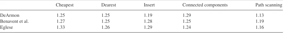
Table 1

Ratios of average solution values to average best solutions for the initial solution methods

Cheapest Dearest Insert Connected components Path scanning

DeArmon 1.25 1.25 1.19 1.29 1.13

Benavent et al. 1.27 1.25 1.28 1.25 1.19

Eglese 1.33 1.26 1.29 1.24 1.16

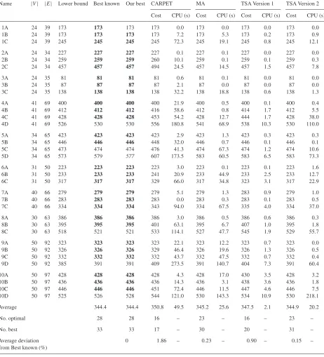
Table 2

Problems from DeArmon[20]

No. |V| |E| Best known Our best CARPET MA TSA Version 1 TSA Version 2

Cost CPU (s)a Cost CPU (s)b Cost CPU (s)c Cost CPU (s)c

1 12 22 316 316 316 2.4 316 0.0 316 0.0 316 0.0

2 12 26 339 339 339 4.0 339 0.3 345 0.1 339 0.1

3 12 22 275 275 275 0.1 275 0.0 275 0.0 275 0.0

4 11 19 287 287 287 0.1 287 0.0 287 0.0 287 0.0

5 13 26 377 377 377 4.3 377 0.1 377 0.0 377 0.1

6 12 22 298 298 298 0.7 298 0.1 298 0.0 298 0.0

7 12 22 325 325 325 0.0 325 0.1 325 0.0 325 0.0

10 27 46 348 348 352 47.2 350 26.5 352 2.5 348 1.6

11 27 51 303 303 317 41.8 303 4.7 307 1.0 303 26.1

12 12 25 275 275 275 1.2 275 0.1 275 0.0 275 0.0

13 22 45 395 395 395 1.8 395 0.9 395 0.2 395 0.1

14 13 23 458 458 458 16.0 458 6.5 462 0.2 458 0.8

15 10 28 536 536 544 1.9 536 4.9 544 0.2 540 4.8

16 7 21 100 100 100 0.4 100 0.1 100 0.0 100 0.1

17 7 21 58 58 58 0.0 58 0.0 58 0.0 58 0.0

18 8 28 127 127 127 1.3 127 0.1 129 0.2 127 0.1

19 8 28 91 91 91 0.0 91 0.1 91 0.0 91 0.0

20 9 36 164 164 164 0.2 164 0.1 164 0.0 164 0.0

21 8 11 55 55 55 0.2 55 0.0 55 0.0 55 0.0

22 11 22 121 121 121 7.4 121 0.2 123 0.1 121 0.2

23 11 33 156 156 156 0.9 156 0.1 156 0.0 156 0.0

24 11 44 200 200 200 2.6 200 2.3 200 0.0 200 0.1

25 11 55 233 233 235 26.6 233 34.1 235 0.7 235 22.3

Average 253.8 253.8 255.0 7.0 253.9 3.5 255.2 0.2 254.0 2.5

No. optimal 23 23 19 – 22 – 15 – 21 –

Average deviation from 0.00 0.47 – 0.04 – 0.55 – 0.08 –

Best known (%)

Optimal solutions are in bold.

a_{The original value has been divided by 7 (SGI Indigo2 at 195 MHz).} b_{The original value has been divided by 1.5 (Pentium III at 1 GHz).} c_{We used a Pentium Mobile at 1.4 GHz.}

(3) recalculatef (SB)with the new value ofP, and empty tabu list.

(Note that the changes to the parameter values and emptying the tabu list at this point means that the sequence of solutions followingSis different to the sequence generated previously.)

7.Stopping criterion:

If (k900√NandkBF10N) orkBT=2kLthenstop, otherwise go to Step 2.

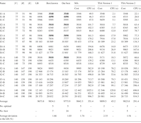
[image:7.544.46.507.191.527.2]

(8)

[image:8.544.40.502.92.601.2]

Table 3

Problems from Benavent et al.[21]

Name |V| |E| Lower bound Best known Our best CARPET MA TSA Version 1 TSA Version 2

Cost CPU (s) Cost CPU (s) Cost CPU (s) Cost CPU (s)

1A 24 39 173 173 173 173 0.0 173 0.0 173 0.0 173 0.0

1B 24 39 173 173 173 173 7.2 173 5.3 173 0.2 173 0.9

1C 24 39 245 245 245 245 72.3 245 19.1 245 0.8 245 12.1

2A 24 34 227 227 227 227 0.1 227 0.1 227 0.0 227 0.0

2B 24 34 259 259 259 260 10.1 259 0.1 259 0.1 259 0.3

2C 24 34 457 457 457 494 24.5 457 14.5 457 1.5 457 7.8

3A 24 35 81 81 81 81 0.6 81 0.1 81 0.0 81 0.0

3B 24 35 87 87 87 87 2.1 87 0.0 87 0.0 87 0.0

3C 24 35 138 138 138 138 32.2 138 18.8 138 0.6 138 1.3

4A 41 69 400 400 400 400 21.9 400 0.5 400 0.1 400 0.4

4B 41 69 412 412 412 416 58.6 412 0.8 414 1.7 412 5.5

4C 41 69 428 428 428 453 54.2 428 12.7 444 1.7 428 38.0

4D 41 69 526 530 530 556 180.8 541 68.9 538 10.3 530 110.0

5A 34 65 423 423 423 423 2.9 423 1.3 423 0.3 423 0.3

5B 34 65 446 446 446 448 32.0 446 0.7 446 0.1 446 0.1

5C 34 65 473 474 474 476 41.3 474 67.3 474 1.2 474 10.6

5D 34 65 573 579 577 607 173.5 583 60.5 583 6.5 583 73.3

6A 31 50 223 223 223 223 3.0 223 0.1 223 0.1 223 1.6

6B 31 50 233 233 233 241 20.9 233 44.9 233 2.5 233 12.7

6C 31 50 317 317 317 329 66.0 317 34.8 323 3.1 317 22.9

7A 40 66 279 279 279 279 5.1 279 1.3 283 0.9 279 1.0

7B 40 66 283 283 283 283 0.0 283 0.3 283 0.1 283 0.5

7C 40 66 334 334 334 343 94.0 334 67.5 335 4.0 334 37.0

8A 30 63 386 386 386 386 3.0 386 0.5 386 0.6 386 0.3

8B 30 63 395 395 395 401 63.1 395 6.7 407 1.0 395 1.8

8C 30 63 518 521 521 533 114.1 527 47.7 545 1.9 529 55.7

9A 50 92 323 323 323 323 22.1 323 12.2 323 0.7 323 0.0

9B 50 92 326 326 326 329 46.4 326 19.6 326 1.3 326 0.5

9C 50 92 332 332 332 332 43.7 332 47.5 332 0.7 332 0.4

9D 50 92 385 391 391 409 273.5 391 140.7 404 7.3 391 60.4

10A 50 97 428 428 428 428 4.3 428 17.0 430 3.5 428 3.2

10B 50 97 436 436 436 436 14.3 436 3.1 438 3.6 436 1.8

10C 50 97 446 446 446 451 72.4 446 11.5 447 4.6 446 7.5

10D 50 97 525 526 528 544 121.0 530 143.3 534 10.9 530 218.1

Average 344.4 344.4 350.8 49.5 345.2 25.6 347.5 2.1 344.9 20.2

No. optimal 28 28 16 – 23 – 16 – 23 –

No. best 33 33 17 – 30 – 20 – 31 –

Average deviation 0 1.86 – 0.23 – 0.90 – 0.15 –

from Best known (%)

In Version 2, the TSA works in four phases. In Phase 1, the TSA is applied to each of the ﬁve initial solutions described in Section 2. In Phase 2, the TSA is applied once more to the best solution from Phase 1, but witht=N/6 and initial values ofFSI=1,FDI=10,FSWAP=3. Phase 3 works as Phase 1, but witht=N/8 and ﬁxed values of

(9)

[image:9.544.42.505.87.490.2]

Table 4

Problems from Eglese

Name |V| |R| |E| LB Best known Our best MA TSA Version 1 TSA Version 2

Cost CPU (s) Cost CPU (s) Cost CPU (s)

E1-A 77 51 98 3548 3548 3548 3548 49.5 3548 2.1 3548 22.1

E1-B 77 51 98 4498 4498 4498 4498 46.3 4533 4.8 4533 28.0

E1-C 77 51 98 5566 5595 5595 5595 47.5 5659 5.1 5595 24.1

E2-A 77 72 98 5018 5018 5018 5018 101.7 5018 7.7 5018 63.4

E2-B 77 72 98 6305 6340 6317 6340 102.3 6385 11.5 6343 66.7

E2-C 77 72 98 8243 8395 8335 8415 86.4 8400 12.0 8347 78.7

E3-A 77 87 98 5898 5898 5898 5898 161.3 6044 17.9 5902 77.3

E3-B 77 87 98 7704 7816 7777 7822 170.2 7916 17.8 7816 113.4

E3-C 77 87 98 10 163 10 369 10 305 10 433 137.6 10 309 23.2 10 309 134.3

E4-A 77 98 98 6408 6461 6456 6461 194.6 6476 14.0 6473 135.5

E4-B 77 98 98 8884 9021 9000 9021 208.6 9134 26.9 9063 167.6

E4-C 77 98 98 11 427 11 779 11 601 11 779 168.3 11 627 31.8 11 627 188.6

S1-A 140 75 190 5018 5018 5018 5018 139.1 5171 10.3 5072 66.6

S1-B 140 75 190 6384 6435 6388 6435 139.2 6388 13.1 6388 80.8

S1-C 140 75 190 8493 8518 8518 8518 110.4 8739 6.9 8535 79.2

S2-A 140 147 190 9824 9995 9956 9995 582.9 10 190 70.2 10 038 395.1

S2-B 140 147 190 12 968 13 174 13 165 13 174 507.0 13 284 78.2 13 178 448.3 S2-C 140 147 190 16 353 16 715 16 505 16 795 498.0 16 709 53.6 16 505 515.8

S3-A 140 159 190 10 143 10 296 10 260 10 296 713.7 10 508 79.3 10 451 554.2 S3-B 140 159 190 13 616 14 028 13 807 14 053 709.3 13 981 84.2 13 981 570.6 S3-C 140 159 190 17 100 17 297 17 234 17 297 582.9 17 346 99.1 17 346 596.4

S4-A 140 190 190 12 143 12 442 12 341 12 442 1025.1 12 546 129.8 12 462 696.8 S4-B 140 190 190 16 093 16 531 16 442 16 531 953.5 16 695 141.4 16 490 954.6 S4-C 140 190 190 20 375 20 832 20 591 20 832 996.7 20 981 144.9 20 733 934.5

Average 9673.8 9834.1 9773.9 9842.3 351.4 9899.5 45.2 9823.0 291.4

No. optimal 5 5 5 – 2 – 2 –

No. best – 7 24 7 – 3 – 5 –

Average deviation – 1.66 1.03 1.74 – 2.33 – 1.54 –

to the LB (%)

Optimal solutions are in bold. New best solutions are in italic.

Phase 2 again to the best solution just found. Finally, Phase 4 applies the TSA to the best solution of the previous phases with the following parameters:t=N/3,kB=25N, and ﬁxed values ofFSI=1,FDI=10,FSWAP=3. Phases 3 and

4 were not applied to the Eglese set of problems, as for these larger problems, the additional computing time required gave only a small improvement.

4. Results of experiments

Computational experiments have initially been conducted on three sets of CARP problems that have been studied in the literature. The ﬁrst set contains 23 instances originally generated by DeArmon[20]and discussed by Golden et al.

(10)

[image:10.544.39.505.86.442.2]

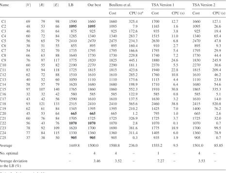
Table 5

Problems from Beullens et al.—set C

Name |V| |R| |E| LB Our best Beullens et al. TSA Version 1 TSA Version 2

Cost CPU (s)a Cost CPU (s) Cost CPU (s)

C1 69 79 98 1590 1660 1660 325.4 1700 12.7 1660 127.1

C2 48 53 66 1095 1095 1095 7.9 1165 1.6 1095 26.6

C3 46 51 64 875 925 925 172.6 935 3.8 925 19.4

C4 60 72 84 1285 1340 1340 283.7 1515 11.0 1340 65.4

C5 56 65 79 2410 2470 2475 234.3 2630 6.8 2470 47.8

C6 38 51 55 855 895 895 160.4 910 2.7 895 9.3

C7 54 52 70 1735 1795 1795 166.6 1795 5.4 1795 29.9

C8 66 63 88 1640 1730 1730 229.8 1740 7.2 1730 44.4

C9 76 97 117 1775 1820 1825 445.1 1880 24.6 1830 245.9

C10 60 55 82 2190 2270 2290 181.1 2370 5.5 2270 30.6

C11 83 94 118 1725 1815 1815 423.6 1940 22.8 1815 209.4

C12 62 72 88 1510 1610 1610 285.2 1760 10.8 1610 46.2

C13 40 52 60 1050 1110 1110 173.6 1115 4.4 1110 23.8

C14 58 57 79 1620 1680 1680 198.9 1710 6.4 1680 54.6

C15 97 107 140 1765 1860 1860 552.3 1910 30.8 1865 335.3

C16 32 32 42 580 585 585 122.9 585 0.8 585 5.1

C17 43 42 56 1590 1610 1610 137.5 1630 3.2 1610 14.0

C18 93 121 133 2315 2410 2410 565.6 2460 38.8 2415 520.8

C19 62 61 84 1345 1395 1395 210.2 1425 7.0 1400 76.2

C20 45 53 64 665 665 665 1.2 795 1.0 665 2.6

C21 60 76 84 1705 1725 1725 326.9 1725 3.7 1725 32.0

C22 56 43 76 1070 1070 1070 2.8 1070 0.1 1070 0.7

C23 78 92 109 1620 1700 1690 381.6 1775 18.9 1700 99.5

C24 77 84 115 1330 1360 1360 311.4 1405 6.0 1360 78.9

C25 37 38 50 905 905 905 0.3 935 1.9 905 0.7

Average 1449.8 1500.0 1500.8 236.0 1555.2 9.5 1501.0 85.85

No. optimal – 4 4 – 1 – 4 –

Average deviation – 3.46 3.52 – 7.27 – 3.53 –

to the LB (%)

a_{The original value on a Pentium II at 500 GHz.}

application in Lancashire[22–24]. There are 24 instances based on two graphs where the different instances have been created by changing the set of required edges and the capacities of the vehicles. Because of the application from which these instances were generated, the demand quantities for the required edges are proportional to their costs.

The full data for these instances can be obtained fromhttp://www.uv.es/∼belengue/carp.html.

To give an impression of the relative accuracy of the ﬁve initial solution methods, the average solution value was calculated for each method over all the instances in each set and this was compared to the average best known solution from the literature over all the instances in each set. The ratios of these averages are given inTable 1. It will be seen that the quality of these initial solutions is poor compared to the ﬁnal solutions generated by the TSA.

(11)

[image:11.544.43.508.86.439.2]

Table 6

Problems from Beullens et al.—set D

D1 69 79 98 725 740 725 11.8 865 2.8 740 62.7

D2 48 53 66 480 480 480 1.2 480 1.6 480 0.8

D3 46 51 64 415 415 415 0.4 415 0.2 415 0.2

D4 60 72 84 615 615 615 0.5 630 4.4 615 1.7

D5 56 65 79 1040 1040 1040 1.4 1080 2.4 1040 2.8

D6 38 51 55 485 485 485 0.2 525 0.7 485 7.9

D7 54 52 70 735 835 835 138.9 915 3.4 835 22.8

D8 66 63 88 615 685 685 195.1 685 4.5 685 49.1

D9 76 97 117 680 680 680 1.1 810 6.1 680 30.1

D10 60 55 82 900 910 910 149.1 910 1.3 910 16.5

D11 83 94 118 920 940 930 368.3 990 8.0 960 112.0

D12 62 72 88 680 680 680 0.4 735 2.5 680 26.0

D13 40 52 60 690 690 690 0.8 695 1.1 695 13.9

D14 58 57 79 920 930 930 180.2 950 1.0 940 21.1

D15 97 107 140 910 950 910 368.8 1100 23.6 950 102.3

D16 32 32 42 170 170 170 0.0 175 0.1 170 0.4

D17 43 42 56 675 675 675 0.2 675 0.0 675 0.0

D18 93 121 133 930 930 930 2.5 1075 13.9 930 190.5

D19 62 61 84 650 680 680 154.8 690 2.7 690 20.1

D20 45 53 64 415 415 415 0.1 420 2.5 415 1.1

D21 60 76 84 695 815 805 251.8 865 2.3 825 60.9

D22 56 43 76 690 690 690 0.3 690 0.0 690 0.0

D23 78 92 109 715 735 735 335.3 780 5.3 735 111.1

D24 77 84 115 620 670 670 248.0 670 10.3 670 105.2

D25 37 38 50 410 410 410 0.0 510 0.2 410 0.6

Average 671.2 690.6 687.6 96.4 733.4 4.0 693.2 38.4

No. optimal 14 15 4 – 13 –

Average deviation – 2.89 2.44 9.27 – 3.28 –

to the LB (%)

the times we recorded for our algorithm. The best results include those reported by Beullens et al.[9], Baldacci and Maniezzo[13]and Longo et al.[14].

InTables 2 and3, if the best known or our best solution is optimal then it is shown in bold. Optimality can be proved for many of the problems in the ﬁrst two sets using the lower bounding procedures described in Belenguer and Benavent[25]. However, these lower bounding procedures still leave a gap between the lower bound and the best known solutions for the larger problems in the third set. Ahr[26], Baldacci and Maniezzo[13]and Longo et al.[14]

have found improvements to some of these lower bounds and the column LB inTable 4gives the best lower bounds found so far for these problems. Note that the lower bounds reported for the second set of test problems in Belenguer and Benavent[25]differ from those reported in Hertz et al.[7]and Lacomme et al.[8]. This is due to a different cost being used for servicing the required edges. As this is a ﬁxed cost incurred by any solution, the consequence is just that a constant term is needed to adjust the results. Details of the adjustments needed are provided in Belenguer and Benavent[25].

The results show that the TSA is capable of providing high quality results. Using the best results from all trials of the TSA with varying swap frequencies and running times, “our best” solutions match the best solutions found for all instances in the ﬁrst set, all instances except the last one in the second set and in the third set of large instances, “our best” solutions are at least as good as the best published results in all 24 instances and in 17 of these instances, a new best solution has been found using the TSA.

(12)

[image:12.544.40.505.86.437.2]

Table 7

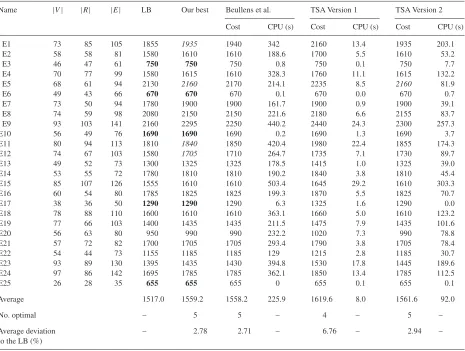
Problems from Beullens et al.—set E

E1 73 85 105 1855 1935 1940 342 2160 13.4 1935 203.1

E2 58 58 81 1580 1610 1610 188.6 1700 5.5 1610 53.2

E3 46 47 61 750 750 750 0.8 750 0.1 750 7.7

E4 70 77 99 1580 1615 1610 328.3 1760 11.1 1615 132.2

E5 68 61 94 2130 2160 2170 214.1 2235 8.5 2160 81.9

E6 49 43 66 670 670 670 0.1 670 0.0 670 0.7

E7 73 50 94 1780 1900 1900 161.7 1900 0.9 1900 39.1

E8 74 59 98 2080 2150 2150 221.6 2180 6.6 2155 83.7

E9 93 103 141 2160 2295 2250 440.2 2440 24.3 2300 257.3

E10 56 49 76 1690 1690 1690 0.2 1690 1.3 1690 3.7

E11 80 94 113 1810 1840 1850 420.4 1980 22.4 1855 174.3

E12 74 67 103 1580 1705 1710 264.7 1735 7.1 1730 89.7

E13 49 52 73 1300 1325 1325 178.5 1415 1.0 1325 39.0

E14 53 55 72 1780 1810 1810 190.2 1840 3.8 1810 45.4

E15 85 107 126 1555 1610 1610 503.4 1645 29.2 1610 303.3

E16 60 54 80 1785 1825 1825 199.3 1870 5.5 1825 70.7

E17 38 36 50 1290 1290 1290 6.3 1325 1.6 1290 0.0

E18 78 88 110 1600 1610 1610 363.1 1660 5.0 1610 123.2

E19 77 66 103 1400 1435 1435 211.5 1475 7.9 1435 101.6

E20 56 63 80 950 990 990 232.2 1020 7.3 990 78.8

E21 57 72 82 1700 1705 1705 293.4 1790 3.8 1705 78.4

E22 54 44 73 1155 1185 1185 129 1215 2.8 1185 30.7

E23 93 89 130 1395 1435 1430 394.8 1530 17.8 1445 189.6

E24 97 86 142 1695 1785 1785 362.1 1850 13.4 1785 112.5

E25 26 28 35 655 655 655 0 655 0.1 655 0.1

Average 1517.0 1559.2 1558.2 225.9 1619.6 8.0 1561.6 92.0

No. optimal – 5 5 – 4 – 5 –

to the LB (%)

halting the programme when a known optimal solution has been found. As expected, Version 1 is faster and the average solution over all the instances in each set only exceeds the best known solution or lower bound on the optimal solution (for the third set) by 0.55%, 0.90% and 2.33%, respectively, for the three problem sets. Version 2 requires longer, but the average solution over all the instances in each set exceeds the best known solution or lower bound on the optimal solution (for the third set) by 0.08%, 0.15% and 1.54%, respectively.

Comparison can be made with CARPET for the first two sets of problems. This shows that the average solution values given by CARPET and Version 1 are very similar, but Version 1 is much faster over all the problems. Version 2 gives slightly better solutions on average than CARPET, finds more best solutions and is still significantly faster.

Comparison can be made with MA for all three sets of problems. Version 1 is much faster than MA, but the results are not quite so good. Version 2 gives results that are slightly better and the computing time is lower than required for MA.

(13)

[image:13.544.41.509.90.440.2]

Table 8

Problems from Beullens et al.—set F

F1 73 85 105 1065 1070 1065 3.4 1090 11.5 1085 88.5

F2 58 58 81 920 920 920 2.3 940 2.6 920 0.3

F3 46 47 61 400 400 400 0.0 480 1.8 400 1.3

F4 70 77 99 930 945 940 247.8 970 2.7 960 63.7

F5 68 61 94 1180 1180 1180 0.2 1185 1.8 1180 17.1

F6 49 43 66 490 490 490 0.0 540 0.4 490 0.0

F7 73 50 94 1080 1080 1080 0.1 1110 3.6 1080 1.7

F8 74 59 98 1135 1145 1145 185.5 1155 1.1 1145 35.7

F9 93 103 141 1145 1155 1145 3.7 1520 7.4 1170 145.9

F10 56 49 76 1010 1010 1010 0.1 1010 0.1 1010 0.1

F11 80 94 113 1015 1015 1015 4.5 1100 8.5 1015 125.8

F12 74 67 103 900 910 910 228.7 1000 4.9 910 47.9

F13 49 52 73 835 835 835 0.2 855 0.8 835 0.2

F14 53 55 72 1025 1035 1025 18.8 1085 2.5 1035 29.7

F15 85 107 126 945 965 945 1.3 1315 22.1 990 145.4

F16 60 54 80 775 775 775 0.1 945 1.9 775 3.4

F17 38 36 50 605 605 605 0.1 660 0.3 630 4.7

F18 78 88 110 835 850 850 274.5 945 13.9 850 92.9

F19 77 66 103 685 725 725 158.0 740 1.5 740 34.9

F20 56 63 80 610 610 610 1.3 610 0.3 610 9.8

F21 57 72 82 905 905 905 4.0 940 2.1 905 45.5

F22 54 44 73 790 790 790 0.4 790 0.1 790 0.4

F23 93 89 130 705 730 725 319.6 895 4.6 730 80.2

F24 97 86 142 975 1010 975 26.6 1040 10.3 1010 79.2

F25 26 28 35 430 430 430 0.1 430 0.0 430 0.1

Average 855.6 863.4 859.8 59.3 934.0 4.3 867.8 42.2

No. optimal – 14 19 – 4 – 13 –

to the LB (%) –

Table 9 Large problems

Name |V| |R| |E| Initial solution cost TSA Version 1

(path scanning method) Cost CPU (s)

G1-A 255 347 375 1 318 092 1 049 708 789.4

G1-B 255 347 375 1 483 179 1 140 692 867.3

G1-C 255 347 375 1 584 177 1 282 270 919.1

G1-D 255 347 375 1 744 159 1 420 126 850.8

G1-E 255 347 375 1 841 023 1 583 133 672.2

G2-A 255 375 375 1 416 720 1 129 229 1455.6

G2-B 255 375 375 1 559 464 1 255 907 1122.3

G2-C 255 375 375 1 704 234 1 418 145 849.0

G2-D 255 375 375 1 918 757 1 516 103 1805.3

G2-E 255 375 375 1 998 355 1 701 681 879.9

[image:13.544.40.509.503.670.2]

(14)

Finally a new set of large instances was created for testing. These were based on a different road network in Lancashire that had been used in a winter gritting study with 255 vertices and 375 edges. Different problem instances were created by changing the set of edges required for service and by changing the capacity of the vehicles.Table 9shows the results from using one of the classical heuristics, the path scanning method, and comparing it with the solution provided by running Version 1 of the TSA. The path scanning method is fast, taking an average of only 0.27 s to ﬁnd a solution. However the TSA improved the results from the path scanning method by 18.5%, taking an average time of 1021.1 s.

5. Conclusions

The paper has demonstrated that the TSA is able to provide high quality solutions to the capacitated arc routing problem (CARP) in a reasonable computing time. Several new best solutions are provided for the Eglese set of test problems that have been studied by other researchers.

The results presented demonstrate the good performance of the TSA compared to CARPET and the memetic algo-rithms approach (MA) of Lacomme et al.[8]. In addition, the TSA is a deterministic algorithm, so all the results are fully reproducible. Both CARPET and MA include several random elements, so different runs of these algorithms may produce different results. CARPET is also complex in the subroutines used within the algorithm. MA is also a complex algorithm and although it has the potential to be easily extended to other problems, it requires many parameters to be set.

The guided local search approach of Beullens et al.[9]describes an alternative deterministic algorithm for solving the CARP. Their approach also provides high quality solutions in a limited computation time. The results show that the TSA is competitive with their approach and has found some new best solutions for the problem instances they introduced.

This paper demonstrates that a relatively straightforward implementation of tabu search (without any long-term memory component or any other procedures to encourage diversiﬁcation apart from different starting solutions and different frequencies for different types of move) is able to produce high quality solutions to the CARP in an efﬁcient manner.

References

[1]Dror M. (Ed.). Arc routing. Theory, solutions and applications. Boston: Kluwer Academic Publishers; 2000.

[2]Lacomme P, Prins C, Ramdane-Cherif W. Evolutionary algorithms for periodic arc routing problems. European Journal of Operational Research 2005;165:535–53.

[3]Lenstra JK, Rinnooy Kan AHG. On general routing problems. Networks 1976;6:273–80. [4]Golden BL, Wong RT. Capacitated arc routing problems. Networks 1981;11:305–15.

[5]Pearn WL. Approximate solutions for the capacitated arc routing problem. Computers and Operations Research 1989;16(6):589–600. [6]Pearn WL. Augment-insert algorithms for the capacitated arc routing problem. Computers and Operations Research 1991;18(2):189–98. [7]Hertz A, Laporte G, Mittaz M. A tabu search heuristic for the capacitated arc routing problem. Operations Research 2000;48(1):129–35. [8]Lacomme P, Prins C, Ramdane-Cherif W. Competitive memetic algorithms for arc routing problems. Annals of Operational Research

2004;131(1–4):159–85.

[9]Beullens P, Muyldermans L, Cattrysse D, Van Oudheusden D. A guided local search heuristic for the capacitated arc routing problem. European Journal of Operational Research 2003;147:629–43.

[10]Greistorfer P. A tabu search metaheuristic for the arc routing problem. Preprint. Amsterdam: Elsevier Science; 2002.

[11]Hertz A, Mittaz M. A variable neighborhood descent algorithm for the undirected capacitated arc routing problem. Transportation Science 2001;35(4):425–34.

[12]Amberg A, Domschke W, Voss S. Multiple center capacitated arc routing problems: a tabu search algorithm using capacitated trees. European Journal of Operational Research 2000;124:360–76.

[13]Baldacci R, Maniezzo V. Exact methods based on node-routing formulations for undirected arc-routing problems. Networks 2006;47:52–60. [14]Longo H, Poggi de Aragão M, Uchoa E. Solving capacitated arc routing problems using a transformation to the CVRP. Computers and Operations

Research 2006;33:1823–37.

[15]Edmonds J, Johnson EL. Matching, Euler tours and the Chinese postman problem. Mathematical Programming 1973;5:88–124. [16]Frederickson GN. Approximation algorithms for some postman problems. Journal of the ACM 1979;26(3):538–54.

[17]Christoﬁdes N. Worst-case analysis of a new heuristic for the traveling salesman problem. Report No. 388, Graduate School of Industrial Administration, Carnegie Mellon University, Pittsburgh; 1976.

[18]Pearn WL, Wu TC. Algorithms for the rural postman problem. Computers and Operations Research 1995;22(8):819–28.

(15)

[20]DeArmon JS. A comparison of heuristics for the capacitated Chinese postman problem. Master’s thesis, University of Maryland, College Park, MD; 1981.

[21]Benavent E, Campos V, Corberán E, Mota E. The capacitated arc routing problem. Lower bounds. Networks 1992;22:669–90. [22]Eglese RW. Routing winter gritting vehicles. Discrete Applied Mathematics 1994;48(3):231–44.

[23]Eglese RW, Li LYO. A tabu search based heuristic for arc routing with a capacity constraint and time deadline. In: Osman IH, Kelly JP, editors. Metaheuristics: theory and applications. Boston: Kluwer Academic Publishers; 1996. p. 633–50.

[24]Li LYO, Eglese RW. An interactive algorithm for vehicle routing for winter-gritting. Journal of the Operational Research Society 1996;47: 217–28.

[25]Belenguer JM, Benavent E. A cutting plane algorithm for the capacitated arc routing problem. Computers and Operations Research 2003;30(5):705–28.