Cosmic Time Transformations in Cosmological Relativity

http://dx.doi.org/10.4236/jhepgc.2016.22022

Cosmic Time Transformations in

Cosmological Relativity

Firmin J. Oliveira

East Asian Observatory, Hilo, HI, USA

Received 10 November 2015; accepted 16 April 2016; published 19 April 2016

Copyright © 2016 by authors and Scientific Research Publishing Inc.

This work is licensed under the Creative Commons Attribution International License (CC BY). http://creativecommons.org/licenses/by/4.0/

Abstract

The relativity of cosmic time is developed within the framework of Cosmological Relativity in five dimensions of space, time and velocity. A general linearized metric element is defined to have the form ds2 = +

(

1 φ

)

c2dt2−dr2+ +

(

1 ψ τ

)

2dv2, where the coordinates are time t, radial distance

r₌ x2₊ y2₊z2 for spatials x, y and z, and velocity v, with c the speed of light in vacuum and _τ the Hubble-Carmeli time constant. The metric is accurate to first order in t τ and v c. The fields

φ and ψ are general functions of the coordinates. By showing that φ ψ= , a metric of the form

s2 c2 t2 r2 2 v2

d = d −d +τ d is obtained from the general metric, implying that the universe is flat. For

cosmological redshift z, the luminosity distance relation DL

( ) (

z t r z

)

t

2 2

, = 1+ 1− τ is used to

fit combined distance moduli from Type 1a supernovae up to z<1.5 and Gamma-Ray Bursts up

to z<7, from which a value of Ω =M 0.800±0.080 is obtained for the matter density parameter

at the present epoch. Assuming a baryon density of Ω =B 0.038±0.004, a rest mass energy of

(

9.79±0.47 GeV

)

is predicted for the anti-baryonic Y and the Φ∗ particles which decay from a hypothetical X₁ particle. The cosmic aging function g₁

( ) (

z t, = 1+z

)

(

1−t2 τ2

)

makes good fits to

light curve data from two reports of Type 1a supernovae and in fitting to simulated quasar like

light curve power spectra separated by redshift ∆ ≈z 1. We determine the multipole of the first

acoustic peak of the Cosmic Microwave Background radiation anisotropy to be l≈224±5 and a

sound horizon of sh0 ≈

(

0.805±0.020

)



θ on today’s sky.

Keywords

1. Introduction

It has recently been reported [1] on the apparent null effect of cosmic time dilation upon light curve power spectra measurements of some 800 low and high redshift quasars (QSO) monitored for 28 years. This appears to contradict two Supernovae Type Ia (SNe-Ia) light curve evolution studies [2] [3] which show the effect of broadening of the power spectra time series consistent with a cosmic time dilation of

(

1+z

)

for redshift z. In this paper, we show that both the QSO and SNe-Ia results are compatible if account is made for the relativity of cosmic time as developed in the theory of Cosmological Special Relativity (CSR) [4]. We also apply these concepts to fitting the combination of high redshift SNe-Ia distance data [5] and Gamma-Ray Bursts (GRB) data

[6].

The Cosmological Relativity of Carmeli [7], the general and special theories, is a five dimensional brane world model based on time t, space x y z, , and velocity v. It makes only one new assumption, that of the maximum value of cosmic time τ which is the Hubble-Carmeli time constant. In the same way that the constant speed of light c constrains the observations in space and time, so too the constant of cosmic time τ constrains the observations of space and velocity. The familiar Lorentz transformations of Einstein Special Relativity (SR) between observers moving at constant relative velocity v carry over into Cosmological Special Relativity (CSR) between observers separated by relative cosmic time t. And just as in SR, there is the special way that velocities add together which reduces to the Galilean form v1+v2 at low velocities with respect to the speed of light, in CSR cosmic times add in an analogous way which has the form t1+t2 for low values with respect to cosmic time τ but is modified for larger cosmic times.

In this paper, we derive only the minimum CSR framework we require for the development of cosmic time transformation effects and the luminosity distance relation. We show that for weak fields φ and ψ (to be defined below), the universe has a flat, Euclidean geometry. And, due to the additive properties of cosmic time in CSR, this gives us a unique form for the luminosity distance relation. We model cosmic time aging effects in light curve data from SNe-Ia. In comparison to the standard Friedmann-Lemaître-Robertson-Walker (FLRW) model, the CGR luminosity distance relation performs quite well in fits to SNe-Ia and GRB distance data, although it requires more dark matter in the mass density. As a consequence, larger rest masses are predicted for the hypothetical X1 particle [8] decay products Y and

*

Φ . We also derive a relation for the first acoustic peak of the Cosmic Microwave Background (CMB) anisotropy.

2. The Universe

The five dimensional Cosmological General Relativity of Carmeli [7] is approximated by the linearized metric element,

(

)

(

)

2 2 2 2 2 2

ds = +1 φ c td −dr + +1 ψ τ d ,v (1) where

2 2 2 2

dr =dx +dy +d .z (2)

The coordinates are time t, spatials x, y and z and velocity v, with c the speed of light in vacuum and τ the Hubble-Carmeli time constant. The linearized model is accurate to first order in v c1 and t τ1. The parameter h=1τ is the Hubble constant at zero distance and no gravity and h≈H0 where H0 is the Hubble constant. The fields φ and ψ are general functions of the coordinates. The CGR standard value for h

is (to three digits) [9],

1 1

72.2 0.84 km s Mpc .

h= ± ⋅ − ⋅ − (3)

This gives

(

)

17

4.28 0.15 10 s 13.6 0.48 Gyr.

τ= ± × = ± (4)

ds=0, (5)

and it is observed at a specific cosmic time t, so that

dt=0. (6) Applying (5) and (6) to (1) yields for the expanding universe

(

)

2 2 2

dr 1 ψ τ dv 0,

− + + = (7)

which reduces to

2 d

1 .

d

r

v ψ

τ

 _{ = +}

 

  (8)

The metric (1) defines the Einstein field equations in five dimensions [7] (Sect. 7.3) 1

, 2

Rν_µ− δν_µR=κT_µν (9)

where Rν_µ is the mixed Ricci tensor [7] (Appendix A), R is the Ricci scalar and T effu u

ν ν

µ =ρ µ is the mixed

energy-momentum tensor, where ρ_eff is the effective mass density and u_µ =uµ =

(

1, 0, 0, 0,1

)

is the velocity vector. The indices ν µ, =0,1, 2, 3, 4 for the five dimensions of _x0 =_{ct x,} 1=_{x x,} 2 =_{y x,} 3 =_{z x,} 4 =τ_v

. The

Kronecker delta δν_µ =1 for µ ν= , and δν_µ =0 for µ ν≠ . The Carmeli gravitation constant κ=8πG c2τ2 where G is Newton's gravitation constant. The 0, 0 component of (9) gives us the equation

0 2

0 1

,

2 eff

R − R=κτ ρ (10)

where

(

) (

)

0 2 2 2

0 ,44 ,00 ,44 ,00

1 1 1

,

2 2 2

R − R= ∇ −φ φ −ψ − ∇ + ∇φ ψ φ− −ψ (11)

2 1

,

2 ψ

= − ∇ (12)

where ψ,00= ∂2ψ ∂t2 and

2 2

,44 v

φ = ∂φ ∂ . From (10) and (12) we get the Poisson equation for cosmology, in the space-velocity domain,

2 2

2 eff.

ψ κτ ρ

∇ = − (13)

The effective mass density is defined by

,

eff c

ρ = −ρ ρ (14)

where ρ is the mass density and ρc is the critical mass density. Under the assumption that the mass is uniformly distributed, the mass density ρ is independent of the spatial coordinate r, but can depend on time t

and velocity v. The critical mass density ρc is a constant defined by

2 3 8π .

c G

ρ = τ (15)

It is useful to express the effective mass density as a parameter in terms of the critical mass density. Dividing by ρc we have

1, eff

eff c

ρ ρ

Ω = = Ω − (16)

of r, the solution to (13) then takes the form ([7], Sect.7.3.2), 2

2 2 2

2 ,

effr GM

c c r

ψ

τ

Ω

= − − (17)

where M is an optional point mass centered at the origin of r. Assuming no central mass, we set M =0. Then putting the expression for ψ from (17) into (8) and simplifying we get

2 2 2 d

1 .

d eff

r

r c

v=τ − Ω τ (18)

3. General Solution in Space-Velocity

The integration of (18) over r and v in the space-velocity domain is carried out at a specific time t. We assume that the mass density ρ is a function of cosmic time only, so that Ωeff will be constant throughout the integration. Substitute Ω − = Ω1 _eff by (16) and put (18) into the integral form

(

)

0 2 2 2 0

d

d .

1 1

r r v

v r c τ τ ′ _′ = ′

+ − Ω

∫

∫

(19)

Integrating (19) and solving for r in terms of v we obtain the general solutions

sinh 1 , for 1,

1

c v

r

c

τ  

= _ − Ω_ Ω <

− Ω   (20)

sin 1 , for 1 and

1

c v

r

c

τ  

= _ Ω − _ Ω >

Ω −   (21)

, for 1.

r=τv Ω = (22)

By use of the identities sinh

( )

i x =isin

( )

x and sin

( )

i x =isinh

( )

x , where x is real and i= −1, we write the general solution as

sinh 1 , for 0 .

1

c v

r

c

τ  

= _ − Ω_ ≤ Ω

− Ω   (23)

4. Flat Space Metric

Equation (17) gave the solution for the field ψ . Now consider the solution for the field φ in (1). The 4, 4 component of (9) gives us the equation [7]

4 2

4 1

,

2 eff

R − R=κτ ρ (24)

where

(

) (

)

4 2 2 2

4 ,44 ,00 ,44 ,00

1 1 1

,

2 2 2

R − R= ∇ψ φ− −ψ − ∇ + ∇φ ψ φ− −ψ (25)

2 1

,

2 φ

= − ∇ (26)

where ψ,00= ∂2ψ ∂t2 and

2 2

,44 v

φ = ∂φ ∂ . Similar to the case for obtaining ψ , we solve (26) to obtain

2

2 2 2

2 ,

effr GM

c c r

φ

τ

Ω

= − − (27)

where M is an optional point mass centered at the origin of r. We see by (17) and (27) that in fact,

( )

r

( )

r ,

φ =ψ (28)

G are part of the (Newtonian) second term. Assuming no central mass (M =0), for the case where the mass density becomes equal to the critical density, ρ→ρc, from (16), the effective mass density parameter

1 0

eff

Ω = Ω − → and the universe becomes Euclidean.

On the other hand, more generally, we can derive a flatspace metric. Given (28), if we divide (1) by 1+ = +φ 1 ψ , we can write

2 2 2 2 2 2

ds =c td −dr +τ d ,v (29) where

d , 1

s s

φ =

+

∫

(30)

and

d , 1

r r

φ =

+

∫

(31)

with the condition that

1 φ.

− < (32)

This implies that for weak fields φ and ψ we can express the cosmology of the expanding universe in

terms of a flat space Euclidean geometry, with a metric of the form ds2=c t2d2−dr2+τ2dv2. In the next section we derive this flat space special theory for cosmology.

5. The Cosmological Special Relativistic Transformation

By (29), with notation r →r, we have the metric

2 2 2 2 2 2

ds =c td −dr +τ d ,v (33) where r is given by (31). The expansion of the universe occurs when ds=0 and observations are made at a particular instant of time t so that dt=0. Then for the expansion, (33) gives us

dr=τd ,v (34)

which, upon integration gives the Hubble law

,

v=rτ =hr (35)

where h=1τ.

In the observable universe there are two classes of objects, those that are bounded by the gravitation of their combined masses and those that are observed to be moving away from one another in the Hubble flow. In other words, if we lump all nearby neighboring galaxies into a super galaxy mass point, then the universe would consist of only super galaxy mass points flying apart in the Hubble flow. Cosmological Special Relativity (CSR) describes these super galactic objects in the universe. However, unlike SR which can have real observers in reference frames which move relatively at less than light speed, in CSR, all galaxies are in the Hubble flow and expand at the Hubble rate h. That is, there are no objects not in the Hubble flow from which to set up a frame of reference and compare observations. Consequently, for CSR we define hypothetical observers in their frames which move relatively at a rate 1t>h. We derive the transformation of coordinates between these hypothetical frames. However, the coordinates of real galaxies are included in the transformation.

vector coordinates

(

τv x y z′ ′ ′ ′, , ,

)

. The magnitude of each 4-vector is defined by

2 2 2 2 2 2 2 2 2_,

S =τ v −x −y −z =τ v −r (36)

2 2 2 2 2 2 2 2 2

,

S′ =τ v′ −x′ −y′ −z′ =τ v′ −r′ (37) with the invariant condition

2 2

,

S =S′ (38)

where r= x2 +y2+z2 and r′= x′2+y′2+z′2. For the case that object O is a galaxy in the expansion, the invariants S2=S′2=0. We refer to S and S′ as 4-vectors even though there are only 2 components, since the 3 spatial components

(

x y z, ,

)

are condensed into _{r= x}2_+y2_+z2

.

To obtain the cosmological transformation ([7], Sect. 2.2), analogous with the Lorentz transformation, assume that a linear transformation exists between the coordinates of hypothetical frames K and K′. In frame K define the space-velocity 4-vector S=

(

τv r,

)

with magnitude

2 2 2 2 0.

S =τ v −r ≥ (39) Similarly, in frame K′ define the space-velocity 4-vector S′=

(

τv r′ ′,

)

with magnitude

2 2 2 2

0.

S′ =τ v′ −r′ ≥ (40) By the requirement that the magnitude of a 4-vector is invariant under transformations between reference frames then

2 2

.

S =S′ (41) Clearly, by (39) and (40), the 4-vectors S and S′ describe coordinates which can be either in the Hubble flow, when 2 2

0

S =S′ = , or not in the Hubble flow, when 2 2 0

S =S′ > . In order to obtain the transformation equations between the 4-vectors it is required that the reference frames K and K′ be separated by a fixed cosmic time of t<τ.

Then, for constants cosh

( )

σ and sinh

( )

σ , where σ is a constant hyperbolic angle, define r′ and v′

such that

( )

( )

cosh sinh ,

r′ =r σ −τv σ (42)

and

( )

( )

cosh sinh .

v v r

τ ′ =τ σ − σ (43)

To solve for the angle σ use the boundary condition r′ =0 which represents the origin of frame K′. At 0

r′ = (42) yields,

( )

sinh

( )

_{( )}

tanh ,

cosh

r t

v

σ σ

σ τ τ

= = = (44)

where

r t

v

= (45)

is the fixed cosmic time separating the origins of frame K′ relative to K. From (44), for ,

t≤τ (46) where t=τ is a limiting condition, we use the hyperbolic functional identities to obtain,

( )

( )

2 2 2

1 1

cosh ,

1 tanh 1 t

σ

σ τ

= =

− − (47)

( )

( )

( )

2 2 2

tanh

sinh .

1 tanh 1

t t

σ τ

σ

σ τ

= =

Substituting from (47) and (48) into (42) and (43) we obtain

2 2, 1 r vt r t τ − ′ =

− (49)

2 2 . 1 v rt v t τ τ τ τ − ′ =

− (50)

By inverting (49) and (50) we get the inverse transform equations

2 2 , 1

r v t r

t τ

′+ ′ =

− (51)

2 2

= .

1 v r t v t τ τ τ τ ′+ ′

− (52)

It can be verified that the transformations (49)-(52) satisfy the invariance requirement of (41) that 2 2

S =S′

by direct substitution into (36) and (37). As was previously mentioned, for a galaxy O with 4-vector S=

(

τv r,

)

observed by the observer in frame K, where 2 2 2 2

0

S =τ v −r = , the transformation Equations (49) and (50) gives for the galaxy O observed in K′ the 4-vector S′=

(

τv r′ ′,

)

where, by the invariance of the transformation, 2 2 2 2

0

S′ =τ v′ −r′ = . Thus, Hubble coordinates are conserved. In the next section we will use this property to obtain the cosmological redshift relation.

6. Cosmological Redshift of Light

We wish to quantify observations of light wave phenomena in the expanding universe made by observers at different cosmic times. Consider the distance r to a galaxy O which is in the Hubble flow, measured by the observer at the origin of K. For the observer at the origin of K′ the distance to the same galaxy O is r′. If r=Nλ and r′=Nλ′, where the λ’s are the measured wavelengths of the light from the galaxy and N is the fixed number of wavelengths, then taking the ratio of distances we get

1 , r N z r N λ λ λ λ = = = +

′ ′ ′ (53)

where z is the cosmological redshift of the light due to the expansion of space during the cosmic time t between frames K′ and K. Substituting for r from (51) into (53) gives

(

)

2 2 , 1

r tv r r

r _{t τ}

′+ ′ ′ =

′ ₋ (54)

2 2 1 . 1 tv r t τ ′ ′ + =

− (55)

For a galaxy which is in the Hubble flow,

1 .

v

r τ

′₌

′ (56)

Substituting from (56) into (55), and along with (53) yields

2 2

1 1

1 .

1 1

r t t

z

r _t t

λ τ τ

λ _τ τ

+ +

+ = = = =

′ ′ ₋ − (57)

Equation (57) is the cosmological redshift of the wavelength of light measured between observers in frames K

and K′. Inverting (57) we get

(

)

(

)

2 2 1 1 . 1 1 z t z τ + − =

7. Dilation of Cosmic Time Due to the Expansion of Space

This transformation is similar to the lengthening of the wavelength of light from a distant galaxy by the factor

(

1+z

)

. From the cosmological redshift relation (57) and the fact that the periods τ_λ and τλ′′ of a wave of light are related to the wavelengths λ and λ′, respectively, by

,

c

λ λ

τ = (59)

,

c

λ λ

τ′ = ′ (60)

we have from (53),

1 ,

N

N c T

z

N c N T

λ

λ

τ λ

λ′ = τ′ = ′= + (61)

where T=τ_λ and T′=τ_λ′. Then the cosmic time dilation from (61) is given by

(

1

)

,

T=T′ +z (62)

where we assume that T′ is an arbitrary time interval in K′.

8. Relativity of Cosmic Time

Dividing (51) by (52) we obtain the transformation for the addition of cosmic time from K′ to K, analogous to the addition of velocities in SR,

1

2 2 2

1 , 1

t t

r r tv

t

v v tr τ tt τ

′

′+ ′ +

= = =

′+ ′ + ′ (63)

where t1′=r v′ ′. The inverse transformation, from K to K′ is obtained by dividing (49) by (50) giving

2

1 2 2

2 , 1

t t

r r tv

t

v v tr τ tt τ

′ − −

′ = = =

′ − − (64)

where t2 =r v. We refer to (63) and (64) as the general cosmic time addition relations. Setting t1′ =τ in (63) yields

2 ₁ 2 ,

t t

t

τ _τ

τ τ

+

= =

+ (65)

implying that two cosmic times can never add up to more than τ . The identical result is obtained from (64) for the time t1′ when t2=τ.

8.1. Contraction of a Small Interval of Cosmic Time in the Past

An increase in cosmic time t by ∆t′ in frame K′ at cosmic time t, where ∆t′τ , will have a value t+ ∆t for the observer in K at cosmic time 0 given by the law of addition of cosmic times (63) by setting t1′= ∆t′ and

2

t = + ∆t t,

2, 1

t t t t

t t τ ′ + ∆ + ∆ =

′

+ ∆ (66)

which yields

2 , 1

t t

t t

t t τ ′ + ∆

∆ = −

′

(

2

)

2 1

, 1

t t t t t

t t τ τ ′ ′ + ∆ − + ∆ = ′

+ ∆ (68)

(

2 2

)

1 ,

t′ t τ

≈ ∆ − (69)

since ∆t′τ. This is a cosmic time contraction of a small time ∆t′ in K′ at cosmic time t measured by the observer in K [10]. It implies that when viewed from the present epoch, a clock will appear to tick more slowly the further back it is in cosmic time. However, this does not alter the physical constants like G, , or e, which remain constants. This is analogous to the case in SR where a clock at the origin of a frame with relative velocity v to the local frame, ticks at the rate δt′ in its own frame but appears to run more slowly at the rate

2 2 1

t v c

δ ′ − when viewed from the local frame, but the physical constants do not vary.

8.2. Dilation of a Small Interval of Cosmic Time in the Present

There is a second kind of effect of time addition which is measured by the observer in K′ situated at cosmic time t from K. Take the cosmic time lapse ∆ = + ∆ −t

(

t t

)

t recorded in K where ∆tτ . What is the observation of that time lapse for the observer in K′? In other words, in K′ what is the difference of the later time t+ ∆t with respect to the earlier time t? The time transformation we use for the K′ frame is from (64) by setting t1′= ∆t′, t2= + ∆t t giving

(

)

(

)

2, 1

t t t

t

t t t τ + ∆ − ′

∆ =

− + ∆ (70)

2 2, 1

t t τ ∆ ≈

− (71)

since ∆tτ. This is a cosmic time dilation of a small time interval in frame K measured in K′. It infers that a short time interval at the present epoch corresponds to a larger time interval further back in cosmic time. Note that if t+ ∆ =t τ then (70) gives ∆ =t′ τ so that we never get a time greater than τ as long as we add times

τ ≤ .

9. Total Cosmic Time Transformation Due to the Expansion of Space

and the Additon of Cosmic Times

Combine the two transformations by taking the product of time dilation (62) due to the expansion of the universe with time contraction (69) due to the addition of cosmic times. The total elapsed cosmic time ∆t observed by the observer in K at cosmic time 0 for a small time change ∆t′τ in frame K′ at cosmic time t

is given by

(

)

(

2 2

)

( )

1

1 1 ,

t z t τ t′ g t t′

∆ = + − ∆ = ∆ (72)

where by substituting for 1+z from (57), the cosmic aging function g t1

( )

is defined by

( )

(

2 2

)

1

1

1 .

1

t

g t t

t τ _τ τ  +  =_{ } − −

  (73)

Substituting for t τ from (58) in terms of redshift z into (73) yields,

( )

(

)

(

)

3

1 ₂ 2

4 1 . 1 1 z g z z + =  _{+ +}    (74)

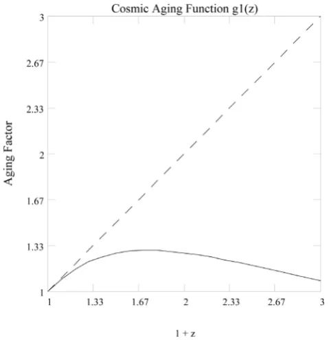
The cosmic aging function g t1

( )

>1 for tτ <0.8392, which gives a time dilation, and g t1

( )

<1 for 0.8395

t τ > , which corresponds to a time contraction. The maximum occurs at t τ =1 2 where

( )

1 2 1.299

g τ = which, from (57), corresponds to a redshift z≈0.732. Figure 1 is a plot of the cosmic aging

[image:10.595.194.434.84.332.2]

Figure 1. Cosmic aging function g z₁

( ) (

=4 1+z

) (

3 _1+z

)

2+1_2, 0< <z 2, solid line. The dashed line is 1+z.

10. Distances

We use the distance relation (23) with the density Ω = ΩM, giving

( )

(

)

sinh 1

1

M

M

c v c

r

τ − Ω

=

− Ω (75)

where ΩM is the average mass density parameter at the present epoch.

In CGR the luminosity distance relation DL includes the contraction of a small interval of cosmic time in the past (69). It enters through the concept that the energy measured over an interval of time ∆t′ from a source with luminosity L at rest in frame K′ at cosmic time t, radiates a proportional quantity of energy E measured by the observer in K given by

(

2 2

)

(

)

( )

1

1 1 ,

E∝L −t τ + ∆ =z t′ L g t ∆t′ (76)

which from (73) is the cosmic aging function g t₁

( )

operating on the time interval ∆t′. Using (76) as the form for the energy of the source in the derivation [10], the luminosity distance DL is given by

(

)

2 2 1

, 1

L

r z

D

t τ + =

− (77)

which is a factor

(

1−t2 τ2

)

−1 2 of the standard form D_L=r

(

1+z

)

, implying that in CGR sources appear less

luminous and thus further away due to the relativity of cosmic time. Substituting for distance r from (75) and for 1+z from (57), and simplifying, (77) becomes

( )

(

( )

)

(

)

sinh 1

.

1 1

M L

M

c v c

D t

t

τ τ

− Ω =

− − Ω (78)

11. Distance Data Fitting

We apply the luminosity distance relation (78) plus a calculated best fit fixed offset aoff to get the apparent magnitude m z

( )

of a distant luminous source,

( )

5 log _L

( )

_{B off},

m z = _D z _+M +a (79)

where we apply (58) to convert from t τ to z in obtaining DL

( )

z . We use the CGR standard value [9] of 4158 Mpc

cτ= . In practice the source absolute magnitude MB is absorbed into the value of the offset aoff . We include in our analysis data from both SNE-Ia and GRB studies. The SNE-Ia data come from the Supernova Cosmology Project SCP Union 2.1 data set [5] of 580 SNe-Ia magnitudes and errors up to z<1.5. The GRB distance data of 69 burst events come from [6] which are selected events up to z<7 from website data provided by [11]. For the mj observed magnitudes and merrj respective errors, the

2

χ for the fit is defined by

( )

2 2

1

. N

j j

j j

m m z

merr

χ

=

 − 

 

=

 

 

∑

(80)

The reduced chi-squared χred2 is given by

(

)

2 2

, 1 red

N k

χ χ =

− − (81)

where N is the number of data samples and k is the number of fitting parameters. For the ΛCDM model the luminosity distance relation is given by

( )

(

)

(

)

0 3

d

1 ,

1 z L cdm

M u

D z c z

u

λ τ

Λ

= +

Ω + + Ω

∫

(82)

where Ω + Ω =M Λ 1 for flat space [12].

Although SNE-Ia data are independent of any particular cosmology, this is not so for GRB data which must be calibrated with a specified cosmological model. This is because SNE-Ia have nearby sources to use for calibration, but for GRB there are no nearby sources for this purpose. The original GRB data set was calibrated with the ΛCDM cosmology. To recalibrate the GRB data for the CGR cosmological model [13] we use the relation

( )

( )

1

( )

_{( )}

log ,

cgr cdm

cdm

DL z

M z M z

DL z

λ

λ

γ

 

= + _{ }

  (83)

where Mλcdm is the original GRB distance modulus calibrated with the ΛCDM model, Mcgr

( )

z is the distance modulus calibrated for the CGR model and γ1 is a conversion factor. The magnitude errors were also converted using (83). We determined a good fitting value of γ =1 1.044442 which was used to convert the GRB distance moduli for all fits to the CGR model. The converted GRB data were combined with the SNE-Ia data to form the complete data set. For the CGR model, the number of parameters k=3 for ΩM, aoff and

1

γ . The parameter τ is fixed in this analysis, so the number of degrees of freedom N_dof = − − =N k 1 645, the same as for the ΛCDM model. The best fit for the CGR model is shown in Table 1 for

0.800 0.080 M

Ω = ± (a conservative estimate of ±10% error) with offset a_off =0.140 and γ =1 1.044442

having a reduced chi-squared χ2 N_dof =1.001182 for N_dof =645. The results are shown inFigure 2. Figure 3shows the histogram of the normalized residual errors for the fit. The solid curve is a Gaussian with mean

0

µ= and standard deviation σ =1 with an amplitude A=135 estimated “by eye” to give a close fit to the histogram. The fit appears good [6] [13] [14].

We fit the ΛCDM cosmology to the original GRB data set, which was calibrated with Ω =M 0.270 and

0.730 Λ

[image:12.595.168.461.83.336.2]

Figure 2. SCP Union 2.1 SNe-Ia data [5] (filled circles) and GRB [6] (dotted x’s). The solid line is for CGR DL z

( )

from (79). The CGR standard value was used for 1τ= =h 72.2 0.84 km s Mpc± . The parameters for the CGR model were the calculated best fit values, with mass density Ω =_M 0.800, offset a_off =0.140 and GRB conversion factor γ₁=1.044442. Magnitude and magnitude errors both were converted to the CGR model (83). For the fit to 649 data points with 3 parameters the reduced

2

1.001182

χ = .

Figure 3. Histogram of CGR residuals mk−m z

( )

k with DL z

( )

k from (79) with redshift zk from

the SCP Union 2.1 SNe-Ia data [5] and GRB data [6], for calculated best fits with mass density 0.800

M

Ω = , offset a_off =0.140 and γ₁=1.044442. The solid line is a standard Gaussian with mean 0

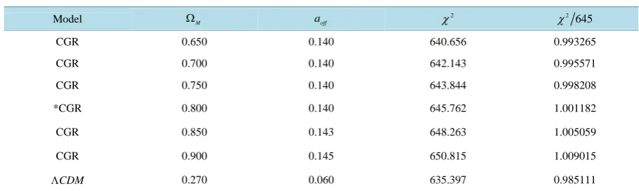
[image:12.595.231.400.434.648.2]

[image:13.595.85.539.149.285.2]

Table 1. CGR vs. ΛCDM model performances with reduced χ2

(

n− −k 1

)

. The number of samples n=649, and

number of parameters k=3 for both models which gives n k− − =1 645. The CGR row showing the best fit is marked with a (*). Refer to the text for an explanation of the best fitting model. The ΛCDM model, with fixed Ω_M and fixed

Λ

Ω has a single best fit for a_off based on the original data.

Model ΩM aoff

2

χ χ2 ₆₄₅

CGR 0.650 0.140 640.656 0.993265

CGR 0.700 0.140 642.143 0.995571

CGR 0.750 0.140 643.844 0.998208

*CGR 0.800 0.140 645.762 1.001182

CGR 0.850 0.143 648.263 1.005059

CGR 0.900 0.145 650.815 1.009015

ΛCDM 0.270 0.060 635.397 0.985111

constant of H0 1τ 72.2 km s1 Mpc1

− −

= = ⋅ ⋅ . The best fit occurred for offset a_off =0.060.Figure 4shows the

Hubble Diagram for the fit of DL cdmλ

( )

z to the combined data, with the GRB moduli used unaltered from the data set. The parameter H0 is fixed in this analysis, so the number of degrees of freedom is the same as for the CGR model. The reduced chi-squared χ2 Ndof =0.985111.Figure 5 shows the histogram of the normalized residual errors for the fit. The solid curve is a Gaussian with mean µ=0 and standard deviation σ =1 with an amplitude A=135 taken from the CGR histogram.

Under the reduced chi-squared statistical model, the ideal reduced 2 1

χ = with the errors distributed normally (Gaussian) about µ=0 with σ =1. The model with a reduced χ2

which is closest to 1 is preferred. Models with reduced 2

1

χ > are deemed to have too few parameters, so “under fit” the data. Models with reduced 2

1

χ < are deemed to have too many parameters and thus “over fit” the data.

We see that the CGR model under fits the data by ≈0.001182, while the ΛCDM model over fits the data by ≈0.014889. For this analysis, the CGR model is ≈10 times better at fitting the combined data. However, considering that we did not vary the mass densities ΩM and ΩΛ, nor the Hubble parameter H0, when fitting with the ΛCDM model, we make this conclusion as mainly a statement of our confidence in the CGR model. A more rigorous analysis of the fitting operation would be required.

Dark Matter and the X Particle Hypothesis

Assume that the mass density Ω = Ω + ΩM B D, that is, composed of baryonic matter ΩB and cold dark matter

D

Ω . For Ω_Bh2≈0.020±0.002 (95% confidence level) [15], with the CGR value h=0.722, this gives

0.038 0.004. B

Ω ≈ ± (84)

Then, for Ω_Mcgr =0.800 0.080± and ΩM cdmλ =0.270±0.013, the CGR model gives a dark matter density of

0.762 0.084, Dcgr

Ω ≈ ± (85)

compared to the ΛCDM model which gives a dark matter density of

0.232 0.017. D cdmλ

Ω ≈ ± (86)

In an extension to the standard model (SM), a hypothetical X particle [8] is theorized to exist, having 2 species, 1

[image:14.595.159.484.82.348.2]

Figure 4. SCP Union 2.1 SNe-Ia data [5] (filled circles) and GRB [6] (dotted x’s). The solid line is for

( )

cdm

DLλ z from (82). The CGR standard value was used for 1τ= =h 72.2 0.84 km s Mpc± . For

the ΛCDM model, with fixed Ω =_M 0.270 and fixed Ω =Λ 0.730, the calculated best fit value for offset a_off =0.060. For the fit to 649 data points with 3 parameters the reduced 2

0.985111

χ = .

Figure 5. Histogram of ΛCDM residuals mk−m z

( )

k for DLλcdm

( )

zk from (82) with redshift zk

from the SCP Union 2.1 SNe-Ia data [5] and GRB data [6], for fixed mass density Ω =_M 0.270 and fixed dark energy mass density Ω =_Λ 0.730, with a calculated best fit offset aoff =0.060. The solid line is a standard Gaussian with mean µ =0 and standard deviation σ=1 and the amplitude factor

135

[image:14.595.222.405.426.641.2]

this extended model, is theorized to be composed entirely of hidden particle states (Y,Φ*). Rare processes can transfer baryonic number from the hidden sector to the visible sector through inelastic scattering of anti-baryonic dark matter states (Y,Φ*), annihilating baryons in the visible sector. The cosmic abundance of remnant Y and

*

Φ particles, with densities given by n_Y and n_Φ*, respectively, is the same as the baryon density nB in the universe today, and thus would have the same abundance ratio as ηB, the baryon to photon (nγ) ratio. That is,

* ₁₀

6 10 ,

Y B

B

n

n n

n_γ n_γ n_γ η

− Φ

= = = ≈ × (87)

for a baryon density Ω ≈B 0.04. Further details of this extension to SM is beyond the scope of this paper. From

[8] (Equation (10)) we can relate the ratio of the density of dark matter (anti-baryonic) to baryonic matter in the universe to the ratio of the rest masses of the Y , _Φ*

and proton by

* 2

2 , p Y

D

B p p

m m wm

w m m Φ + Ω = ≈ =

Ω (88)

where m_Y and m_Φ* are, respectively, the Y and

*

Φ particle rest masses and m_p is the proton rest mass

and we assumed that mY ≈mΦ* ≈wmp. For the CGR model, (88) yields

0.762 0.084 2 , 0.038 0.004 Dcgr cgr B w

Ω ₌ ± ₌

Ω ± (89)

which implies

10.43 2.18. cgr

w = ± (90)

This gives rest mass energies for the Y and Φ* particles of

(

)

*

2 2

9.79 0.47 GeV. Ycgr cgr

m c m c

Φ

≈ ≈ ± (91)

For the ΛCDM model, (88) yields

0.232 0.017 2 , 0.038 0.004 D cdm cdm B w λ λ Ω ± = =

Ω ± (92)

which implies

2.61 0.55. cdm

wλ = ± (93) This gives rest mass energies for the Y and _Φ*

particles [8] of

(

)

*

2 2

2.45 0.47 GeV.

Y cdm cdm

m_λ c ≈m_Φλ c ≈ ± (94)

In both cases above we have tried to account for the constraint that mY −mΦ* <mp +me, where me is the electron mass, by restricting the range of values to be within ±0.47 GeV. This may be only an approximate treatment, at best.

12. Time Dilation in SNe-Ia Light Curves

We now consider two SNe-Ia (SNe) light curve experiments [2] [3]. Common to both experiments is the stretch of the SNe light curve interval for each distant source when compared to the standard nearby (local) source. Because these studies rely on a model for what the light curve looks like in the rest frame of the source SNe, we will require the use of both kinds of cosmic time additions described above. The light curve time interval

obsspec

t′

∆ from the distant SNe will be observed to have a time transformation which is a combination of cosmic time addition in the past combined with the time effect of the expansion of space, having the observed value

obs

t

∆ which is given by (72),

(

)

(

2 2

)

1 1 .

obs obsspec

t t′ z t τ

In CSR this is the time interval that is observed from a source light curve or any time varying phenomenon at a cosmic time t in the past.

On the other hand, we can describe the light curve recorded by the observer in the frame K′ at cosmic time t

relative to our local observer in K at cosmic time 0. A light curve time duration of ∆tspec in K, from (71) for a cosmic time addition in the present, corresponds to the value ∆t_spec′ in K′ given by

(

2 2

)

.

1 spec spec

t t

t τ ∆ ′

∆ =

− (96)

If we make the assumption that

, obsspec spec

t′ t′

∆ = ∆ (97)

then combining (95) with (97) yields

(

1

)

.

obs spec

t t z

∆ = ∆ + (98)

It is evident that CSR, assuming (97), is consistent with the time dilation reports showing effects of cosmic aging equivalent with 1+z for redshift z. However, to offer a different perspective on cosmic time transformation, we will show plots of the ratio ∆tobs ∆tobsspec′ given by (95), instead of ∆tobs ∆tspec which was used in those reports.

For the SNe data from [2] the light curve agings are given as the light curve width w and the error in the width w

σ , obtained directly from [2] (Table 1) for the SCP high z SNe and from [2] (Table 3) for the Calán/Tololo low

z SNe. Since the goal of the experiment was to normalize each light curve to a single standard light curve, we will assume that the equivalent local rest frame time is ∆t_spec =1 which implies from (96) that

(

2 2

)

1 1 spec

t′ t τ

∆ = − . The reduced observed quantity is

w

and we will assume using (98),

(

1

) (

1

)

.

obs spec

t t z z w

∆ = ∆ + = + = (99)

We will use (99) to acquire the redshift z and hence t τ from the light curve rather than using the redshift from the host galaxy. The quantity we use is the ratio ∆t_obs ∆t_obsspec′ from (95),

(

)

(

2 2

)

1 1 .

obs

obsspec

t

z t

t τ

∆ _{= + −}

′

∆ (100)

The plotted data are shown inFigure 6. For data points with w<1 the redshift was set to z=0. The plot shows the reduction of apparent light curve aging at higher redshift. This is the effect which would be seen in the observed light curve without scaling by the rest frame aging rate. The reduced chi-squared is χ2 57=10.8

for the data fitted to the cosmic aging rate g1

( )

z , (74).

The next SNe data are from [3]. We take the aging rates

(

∆t_spec ∆t_obs

)

from [3, Table 3], in the last column, unparenthesized. We compute

(

)

(

2 2

)

1 .

obs

obs spec obsspec

t

t t t

t τ

∆ _{= ∆ ∆ −}

′

∆ (101)

The errors come from [3] (Table 3), in the last column, parenthesized. The redshifts are computed from the aging rate data instead of from the given host galaxy values. The plotted data are shown inFigure 7. Again we note the reduction in the aging rate at higher redshifts. The reduced chi-squared for the data fitted to the cosmic aging rate g1

( )

z is

2

34 0.690

χ = . InFigure 8 we show the combination of all the SNe aging data from the two reports. With 93 total data points the reduced chi-squared is χ2 92=6.98.

13. Simulation of Quasar Like Light Curve Power Spectra

[image:17.595.126.496.84.353.2]

Figure 6. Calán/Tololo low z and SCP high z SNe-Ia light curve time intervals [2] (Goldhaber, et al.). Open circles are ∆t_obs ∆t′_obsspec for each of the 58 SNe-Ia. Error bars are computed from the σw data

errors. The solid line is the cosmic aging function g z1

( )

of (74). The reduced 2

χ for the fit of

( )

1

g z to the data is 2

57 10.8

χ = .

Figure 7. SCP low z and high z SNe-Ia light curve time intervals [3] (Blondin, et al.). Filled circles are

obs obsspec

t t′

∆ ∆ for each of the 35 SNe-Ia. Error bars are computed from the data errors. The solid line

is the cosmic aging function g z1

( )

. The reduced 2

χ for the fit of g z1

( )

to the data is 2

34 0.690

[image:17.595.142.491.376.660.2]

[image:18.595.159.473.83.258.2]

Figure 8. Combined SNe-Ia light curve time intervals ∆t_obs ∆t′_obsspec. Open circles are from

[2] (Goldhaber, et al.). Filled circles are from [3, Blondin, et al.]. The solid line is the cosmic aging function g z1

( )

. The reduced

2

χ for the fit of g z1

( )

to the combined

data is 2

92 6.98

χ = .

spectra [1] (Figure 5, left-hand panel) were found to be identical within the experimental errors. Therefore, we will assume the low and high redshift light curves are identical in the observer frame K. In addition, it is assumed that the redshifts are of pure cosmological origin, with no components of gravitational redshifts or Doppler shifts. In our simulation, the pseudo quasar light curve apparent magnitudes m j

( )

at epoch j is generated by the function

( )

2π 2 800 0 2 200 0

exp cos sin ,

y e e

f j f j

j m j

N N N

     

= _− _    

   

  (102)

for each epoch j=1, 2,,Ne , where Ne=560, Ny=56 years and

1 0 1 16.3 yr 0.0613 yr

f = = − . The

redshifts used are low z=0.765 and high z=1.711 and f01 16.3 yr − ₌

are from the quasar time dilation

report [1]. For better resolution we used N_y =56 yr instead of the 28 yr which was used in the report. The Fourier power spectrum P_S

( )

z j, is determined from the magnitudes m j

( )

by [1] (Equation (1))

( )

( )

( )

( )

( )

2 2

1, 1,

2π 2π

, cos sin ,

e e

S

k N k N

e e e e

T z jk T z jk

P z j m j m j

N = N N = N

     

= _{  } + _{  }

   



∑

 

∑

 (103)

where j runs over Ne equally spaced epochs of simulated data separated by time T z

( )

Ne. Then the time transformations will take us from the origin of observer frame K to the quasar rest frame K′ at cosmic time t. For CSR the sampling interval T z

( )

we use is defined by

( )

_{( )}

0 1

,

T T z

g z

= (104)

where g1

( )

z is given by (74) and

0 1 0.

T = f (105)

We divide by g1

( )

z in (104) because we are going back in time to the quasar rest frame.

( )

0 _, 1

T T z

z =

+ (106) where we have again divided out the time transformation to get to the quasar rest frame.

For either model we use the fitting function P f z

(

,

)

defined by [1], Equation (2)

(

)

( )

(

)

0

(

( )

)

, _{a b},

c c

C P f z

f f z f f z −

=

+ (107)

where C0 is the power, f is the frequency, fc

( )

z is the redshift dependent frequency at maximum power and

a and b are constants. We use the appropriate form of fc

( )

z for the CSR or the FLRW models. We show light curve power spectrum plots of log

(

P_S

( )

z j, × f_j

( )

z

)

vs. log

(

f_j

( )

z

)

for the light curves at low and high

redshift.

Assuming both quasars have identical power spectra in the observer frame K, we obtain the power spectrum from (103) by setting the redshift z=0 which is given by P_S

( )

0,j . This is shown inFigure 9 with the fitting power function P_f

(

f z,

)

parameters C0=0.020524, fc

(

z=0

)

=2.4f0, a=1.4α where α =0.81 from

[1] (Table 1, Observer frame Sample = z < 1, Index = −0.81) and b=a. This can be compared with [1] (Figure 5, left-hand panel).

Next we show the light curve power spectra for the low and high redshift quasars, zlow =0.765 and high 1.711

z = , respectively, as it would be observed in their rest frame. The light curves are corrected by

( )

1

[image:19.595.217.411.379.623.2]

1 g z since we are obtaining the light curve back in time. We show the quasar power spectrum along with the fitting function P_f

(

f z,

)

, which has the same parameters as were used at the origin of K except for the frequency at maximum power which is given by

Figure 9. Simulated quasar light curve power spectrum, filled circles, observed at origin of frame K at cosmic time t=0. Low redshift and high redshift quasar power spectra overlap so are shown as one spectrum. The frequency f is 1

yr− . The abscissa (horizontal) axis is

( )

log f and the ordinate (vertical) axis is log power

(

×f

)

. Both axes have unit scaling.

The function Pf

( )

f , solid line, was fitted iteratively with parameters C0=0.020524,

( )

1

0 0.14724 yr

c

( )

2.4 0 1

( )

,

c

f z = f g z (108)

with g₁

( )

z from (74). This is plotted in Figure 10. The fitting function has the same parameters for both the

low and high redshift spectra as were used in the spectrum at the origin of K except for fc

( )

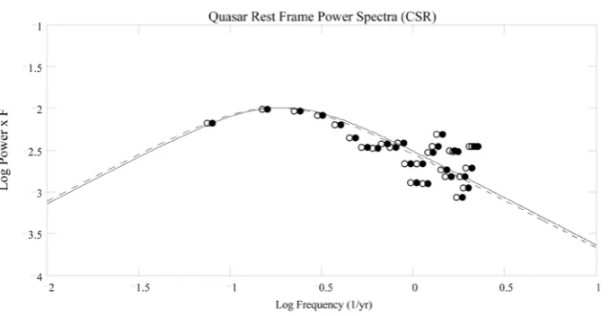
z .

To show what the power spectra might look like for a flat space FLRW observation we show the low and high redshift quasar light curve power spectra when the light curves are corrected for time dilation by 1 1

(

+z

)

, assuming a flat space cosmology. This is shown in Figure 11. This plot is similar to [1] (Figure 5, right-hand panel). The fitting function P_f

(

f z,

)

has the same parameters for both the low and high redshift spectra as were used at the origin of K except for the frequency at maximum power which is given by

( )

2.4 0

(

1

)

.

c

f z = f +z (109)

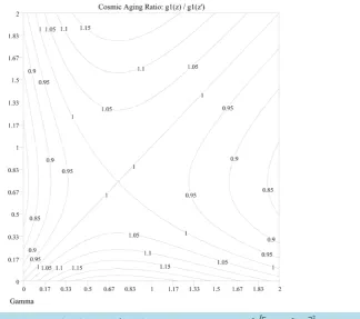
In Figure 12we show a contour plot of the cosmic aging ratio Γ ,

(

z z′

)

defined by

(

)

1

_{( )}

( )

1

, g z ,

z z

g z

′

Γ =

′ (110)

between two source fields, one at redshift z and the other at redshift z′. This is to demonstrate that it is possible to obtain similar aging rates (eg. within 10%) between two sources separated by large redshift. For the above low and high redshifts, Γ

(

1.711, 0.765

)

=0.8803.

For another demonstration of the cosmic aging ratio, we show in Figure 13 the power spectrum for each quasar in its rest frame where z1=0.7 and z2 =1.4. The aging ratio is Γ

(

z z2, 1

)

=0.9317.

14. CMB Anisotropy Acoustic Peak

In CGR the big bang occurred at velocity v=c. At the recombination of protons and electrons in the baryon-photon plasma, when the photons decoupled to form the CMB radiation field, the velocity was v=vrc,

Figure 10. Simulated quasar light curve power spectra in the rest frame K′ of each quasar where each light curve transforms according to CSR. The frequency f is yr−1. For the low redshift power spectrum, filled circles, zlow=0.765, the

horizontal axis is scaled by g z1

( )

low with g z1

( )

from (74) and the vertical axis has unit scaling. The power spectrum

time interval is transformed by 1g z1

( )

low and the frequency is scaled by g z1

( )

low which effectively sets the scale to unity.

For the high redshift power spectrum, open circles, zhigh =1.711, the horizontal axis is scaled by g1

( )

zhigh and the vertical

axis has unit scaling although the power spectrum time interval is transformed by 1 g1

( )

zhigh and the frequency is scaled by

( )

1 high

g z . The fitting function Pf

( )

f has the same parameters as used at the origin of K except the central frequency is

[image:20.595.145.485.417.585.2]

[image:21.595.163.468.85.266.2]

Figure 11. Simulated quasar light curve power spectra in the rest frame K′ of each quasar where each light curve transforms according to flat space FLRW. The frequency f is 1

yr− . For the low redshift power spectrum, filled circles,

low 0.765

z = , the horizontal axis is scaled by 1+zlow. and the vertical axis has unit scaling. The power spectrum time

interval is transformed by 1 1+z_low and the frequency is scaled by 1+z_low which effectively sets the scale to unity. For the high redshift power spectrum, open circles, z_high=1.711, the horizontal axis is scaled by 1+z_high and the vertical axis has unit scaling although the power spectrum time interval is transformed by 1 1+zhigh and the frequency is scaled by

high

1+z . The fitting function Pf

( )

f has the same parameters as used at the origin of K except the central frequency is

scaled by fc

( )

z =0.14724× +

(

1 z

)

with z=zlow, solid line, and z=zhigh, dashed line.

Figure 12. Contour plot of Gamma

( )

z z, ′ =g z1

( ) ( )

g z1 ′ where

( ) (

) (

)

2

3 2

1 4 1 1 1

[image:21.595.183.508.399.686.2]

[image:22.595.147.487.81.257.2]

Figure 13. Simulated quasar light curve power spectra in the rest frame K′ of each quasar, assuming each light curve transforms according to CSR. The frequency f is 1

yr− . For the low redshift power spectrum, filled circles, z₁=0.7, the horizontal axis is scaled by g z1

( )

1 and the vertical axis has unit scaling. The power spectrum time interval is transformed

by 1g z1

( )

1 and the frequency is transformed by g z1

( )

1 which effectively makes the scale unity. For the high redshift

power spectrum, open circles, z2=1.4, the horizontal axis is scaled by g z1

( )

2 and the vertical axis has unit scaling

although the power spectrum time interval is transformed by 1g z1

( )

2 and the frequency is scaled by g z1

( )

2 . The fitting

function Pf

( )

f has the same parameters as used at the origin of K except the central frequency is scaled by

( )

0.14724 1

( )

c

f z = ×g z with z=z1, solid line, and z=z2, dashed line.

which is related [4] to the time trc of recombination by vrc c=trc τ . Applying (58), we have

(

)

(

)

2

2

1 1

,

1 1

rc rc rc

rc

z

v t

c τ z

+ −

= =

+ + (111)

where zrc is the cosmological redshift at recombination. The coordinate distance rbb to the big bang is given by (23) with v c=1,

(

)

sinh 1 .

1

bb M

M

c

r = τ − Ω

− Ω (112)

Likewise, the coordinate distance rrc to the recombination epoch with v c=vrc c, is given by

sinh 1 .

1

rc

rc M

M

v c

r

c

τ  

= _ − Ω _

− Ω   (113)

We construct a simple model to determine the size of the sound horizon [16] [17] for the longest sound wave, which generates the first acoustic peak. If re is the radius of the sphere of expanding plasma, ve=

(

c+vrc

)

2 is the average expansion velocity between the big bang and the recombination epoch and cs=c 3 is the

speed of the longest sound wave in the plasma, then, by proportion of velocities, rsh =

(

c v rs e

)

e is the radius of the sphere containing the longest wave. Assuming that the wave travels along a great circle path of the sphere, the size of the sound horizon dsh is given by

(

)

4π

2π .

3 1 e

sh sh

rc r

d r

v c

= =

+ (114)

(

)

(

)

(

)

(

)

sinh 1 sinh 1

4π 4π

. 1

3 3 1 1

M rc M

bb rc

sh

rc M rc

v c

r r c

d

v c v c

τ   − Ω −  − Ω 

−     

= ₊ =  

− Ω +

 

 

(115)

The angle θsh of the sound horizon at recombination is given by

, sh sh rc d DA

θ = (116)

where the angular diameter distance DArc is given by [10]

(

)

2, 1 rc rc rc DL DA z =

+ (117)

where DLrc is the luminosity distance of the recombination epoch. Substituting from (111)-(115) and (117) into (116) and simplifying we obtain

(

)

(

)

2 2 _{sinh 1}

1 1

4π

1 . 1

3 sinh 1

M

rc rc

sh

rc rc M

z t

v c v c

τ

θ =  + − _  − Ω  − _

+  

 _ − Ω _

    

(118)

The CMB radiation escaped the matter sphere and expanded to fill all space. The size of the sound horizon

0 sh

d in the CMB on today’s sky is obtained by applying (53) with dsh,

(

)

0 1 .

sh sh rc

d =d +z (119)

Then, the angle θsh0 of the sound horizon in the CMB radiation field on today's sky is given by

(

)

0

0 1 .

sh

sh sh rc

rc

d

z DA

θ = =θ + (120)

The multipole l of the first acoustic peak [16] recorded in the CMB radiation field is proportional to the inverse of (120),

(

)

0

π π

. 1

sh sh rc

l

z

θ θ

≈ =

+ (121)

Substituting Ω =M 0.800±0.080 and zrc =1100 into the above equations we obtain a value of 224 5,

l≈ ± (122)

which is in good agreement with observation [18] [19] and,

0 0.805 0.020 . sh

θ ≈ ±  ₍₁₂₃₎

The size of the sound horizon on today’s sky is dsh0≈30.2 Mpc, which is 1/5 the value of the standard model.

15. Discussion

Let us review briefly some aspects of the Carmeli five dimensional brane world cosmological model.

15.1. Velocity, Acceleration and Cosmic Distances in CSR

From (33), for dt=0 with dx2+dy2+dz2=dr2 we have,

(

)

2 2 2 2 2 2

ds =τ dv − dx +dy +dz , (124)

This can be manipulated to obtain

2 2 2 2 2 2

2 2

2 2 2

d d d d d

1 1 1 ,

d d d

v x y z v t

s v s

τ τ

τ τ

 + +   

   

= _{  } − _= _{  } − _

  _{ }   _{ } (125)