Munich Personal RePEc Archive
Structural Models and Endogeneity in
Corporate Finance: the Link Between
Managerial Ownership and Corporate
Performance
Coles, Jeffrey and Lemmon, Michael and Meschke, Felix
University of Minnesota
15 February 2007
Structural Models and Endogeneity in Corporate
Finance: The Link Between Managerial Ownership
and Corporate Performance
Jeffrey L. Coles, Michael L. Lemmon, and J. Felix Meschke*
First version: July 3, 2002
This version: February 15, 2007
*An earlier version of this paper was titled “Structural Models and Endogeneity in Corporate Finance”.
Structural Models and Endogeneity in Corporate Finance: The
Link Between Managerial Ownership and Corporate Performance
ABSTRACT
This paper presents a parsimonious, structural model that captures primary economic determinants of the relation between firm value and managerial ownership. Supposing that observed firm size and managerial pay-performance sensitivity (PPS) maximize value, we invert our model to panel data on size and PPS to obtain estimates of the productivity of physical assets and managerial input. Variation of these productivity parameters, optimizing firm size and compensation contract, and the way the parameters and choices interact in the model, all combine to deliver the well-known hump-shaped relation between Tobin’s Q and managerial ownership (e.g., McConnell and Servaes (1990)).
Our structural approach illustrates how a quantitative model of the firm can isolate important aspects of organization structure, quantify the economic significance of incentive mechanisms, and minimize the endogeneity and causation problems that so commonly plague empirical corporate finance. Doing so appears to be essential because, by simulating panel data from the model and applying standard statistical tools, we confirm that the customary econometric remedies for endo-geneity and causation can be ineffective in application.
The analysis of the relation between firm performance and managerial ownership represents a substantial and consistently-active segment of the empirical corporate finance literature. Important early contributions include Morck, Shleifer, and Vishny (1988), hereafter MSV, which documents a nonmonotonic relation between Tobin’s Q and managerial stock ownership,1 and McConnell and Servaes (1990), hereafter MS, which reports an “inverted-U” or “hump-shaped” relation between
Qand managerial ownership. Numerous successors investigate the ownership-performance relation using different data, various measures of performance and ownership structure, and alternative empirical methods.2
One possible interpretation of the data is that shareholders maximize firm value if they can in-duce managers to own precisely the amount of stock associated with the peak of the performance-ownership relation. For example, based on McConnell and Servaes (1990, Table 1, Panel (B), regression (1), 1986 data), maximum Q requires about 37.5 percent inside (officers and directors) ownership. But if 37.5 percent managerial ownership maximizes value, why would other combi-nations of managerial ownership and Q appear in the data? One obvious possibility is that large transaction costs prevent a firm from moving to the optimum. Only when the distance away from the optimum is large will the benefits to shareholders of realigning ownership structure exceed the transaction costs of doing so. Within the bounds of those costs the data would trace the objective function that the firm would maximize in the absence of such costs.3
In our data, ownership of the CEO varies from 0.01% to 57.6%, with a standard deviation
1 Choosing the kink points to best fit the data, MSV find a positive relation between Qand inside ownership
over 0 percent to 5 percent of outstanding shares, a negative relation over the 5 percent to 25 percent range, and a positive relation once again for managerial holdings exceeding 25 percent.
2See Demsetz and Lehn (1985), Kole (1995), Cho (1998), Himmelberg, Hubbard, and Palia (1999),
Dem-setz and Villalonga (2001), Palia (2001), and Claessens, Djankov, Fan, and Lang (2002), among others. The extent of interest in the performance-ownership relation is documented by H. Mathiesen, whose website (http://www.encycogov.com/A5OwnershipStructures.asp) catalogs approximately 100 academic studies on the topic published up through 1999. Many other papers on the topic have appeared since.
3 See Stulz (1988) for a model containing offsetting costs and benefits of managerial ownership. In that model,
of 5.65%, and the point at which the maximum of the hump-shaped relationship between Q and ownership appears in our sample is 20.09%. Based on our estimates of theQ-performance relation, increasing CEO ownership by one standard deviation, from 14.41% to 20.06% implies an increase in firm value equal to $659 million on average. It seems implausible that the transaction costs of realigning CEO pay-performance sensitivity exceed that figure, much less the even greater amounts associated with larger departures of ownership from that which supports maximalQ. Based on this line of reasoning and plausible transaction costs, there is far more variation in observed ownership structure than one would expect.
An alternative interpretation is that the inverted-U pattern represents a value-maximizing rela-tion between two endogenous variables. Under this view, if the empirical specificarela-tion adequately captures the effects of all relevant exogenous variables, i.e. those structural parameters that drive both ownership and performance, that specification would be unlikely to detect any remaining re-lation between the jointly-determined endogenous variables (Demsetz and Lehn (1985)). Thus, one challenge for those who operate in the equilibrium paradigm, in this particular empirical context or any other, is to specify and estimate a structural model of the firm. Doing so offers the potential for understanding how exogenous factors that capture the relevant economic forces associated with the contracting environment operate to give rise to a relation between managerial ownership and firm performance.
value-maximizing managerial ownership and investment from the model to firm data from Execu-comp and Compustat. In particular, for each firm-year observation, we estimate the productivity parameters for managerial input and investment that would give rise to the observed levels of ownership and investment as optimal choices in our model.
We confront the model with several classes of empirical tests. From least to most formal, first we find that the model is invertible - that is, the model is sufficiently flexible to accommodate what appears in the data. There always exist productivity parameters for physical assets and managerial input that support observed firm size and CEO pay-performance sensitivity as optimal.
Second, our estimates of managerial input versus physical capital appear to be significantly different across industries and vary as might be expected. For example, the relative productiv-ity of managerial input compared to capital is high in personal and business services (including educational services, software development, and networking services) and business equipment (in-cluding computers) and low in metal mining and utilities. In the cross-section of industries, CEO pay-performance sensitivity is larger and firm size smaller when our measure of productivity of managerial input is high relative to measured productivity of capital.
Third, we examine whether the productivity parameters and our estimate of Q based on the model (call it Q∗) are correlated with actual Q and operating characteristics of the firm. We
find that the correlations between model-generated Q∗ and R&D intensity, sales, leverage, and
advertising effort are statistically significant and have the same sign as the correlations with actual
Q. Additionally,Q∗ has significant power to explain actual Q(t = 8.79).
Finally, we examine the performance-ownership relation. The model produces the inverted-U relation when we regress Q∗ on CEO ownership (t = 20.09) and its square (t = -14.12). Moreover,
actualQon the two ownership variables (linear and quadratic), but also including on the right hand side simple transformations of the productivity parameters generated by our model, the productivity parameters displace almost all of the explanatory power normally supplied by CEO ownership (t = 1.19) and its square (t = -1.09). Thus, these exogenous structural parameters appear to capture some of the economic forces that determine jointly Tobin’s Q and optimal contract form.
To supplement these results, we evaluate the statistical and economic relevance of the endo-geneity problem in this empirical context. In particular, we generate a panel of data supposing that our model is the true model and that our estimated exogenous productivity parameters are correct. In this simulated data set, ignoring what we know about the true model that generates the data, we find that misspecified regression models continue to yield a relation between performance and ownership that is similar to that documented in McConnell and Servaes (1990). When using firm size (assets or sales), leverage, R&D expense, advertising expense, and industry to proxy for the structural productivity parameters, the spurious relation betweenQand managerial ownership typically remains. These variables are ineffective instruments for the joint determinants of perfor-mance and contract form. Furthermore, we find that there are significant concerns associated with the use of fixed effects that are meant to control for unobserved heterogeneity in the contracting environment. Finally, we present evidence on the efficacy of specifying and estimating a system of simultaneous equations (2SLS). In the end, based on our simulated panel, we find that endogeneity can be a severe problem and that standard approaches used in the literature often fail to provide a solution, unfortunate conclusions which provide further impetus for application of a structural approach.
In broad terms, our analysis makes two classes of contributions. First, we provide an equi-librium explanation for an important and oft-examined empirical finding. In our framework, the
pro-ductivity of physical assets and managerial input. Though our model has a minimal number of elements, it appears to capture some of the essential economic factors that determine contract form, the boundaries of the firm, and market value, all in a way that is consistent with an important empirical regularity.
Second, the methodological implications of our analysis suggest research opportunities in empir-ical corporate finance. Our model is consistent with recent calls by Zingales (2000) and Himmelberg (2002), among others, for a quantitative theory of the firm that is empirically implementable and testable and that allows an assessment of the economic significance of various dimensions of the organization. Moreover, our approach can avoid the endogeneity and causation problems that com-monly plague empirical corporate finance. Doing so is essential because, by simulating data from the model, we illustrate the difficulty of controlling for endogeneity and assessing causation using standard approaches often applied in this empirical context.
The remainder of the paper is organized as follows. Section 1 presents and analyzes a principal-agent model augmented by an investment/scale choice. Section 2 describes our sample. Section 3 describes our empirical strategy. In Section 4, we invert the model to data on managerial ownership and total assets, provide values for parameters that reflect the marginal productivity of managerial input and physical capital, and characterize the economic importance of changes in the structural parameters for investment, ownership, and our proxy for Tobin’s Q. Section 5 examines variation across industries in the productivity parameters andQ∗. We also report the results of our analysis
1.
A Parsimonious Model of Ownership and Investment
Our model is an adaptation of the standard principal-agent problem (see Holmstr¨om (1979) and Holmstr¨om and Milgrom (1987), for example). In particular, the principal chooses the size of the firm as well as the ownership stake (compensation scheme) of the manager. In this model, share-holders choose both the wage contract and firm scale. While it is standard to think of shareshare-holders choosing the managerial compensation scheme, perhaps it is more familiar to think of managers choosing investment. To the extent that investment in physical assets is observable by shareholders, however, it is equivalent to place the decision rights over investment with shareholders.
Firm cash flow is defined by
˜
f ≡pIygz+Ixε˜ (1)
where I is the firm’s investment, or assets, and g is the manager’s input. This input represents productive activities, such as effort, that the manager is reluctant to supply otherwise. Assets (I) can include property, plant, and equipment as well as various intangible assets. Managerial input and investment interact in the production function with parametersy∈(0,1) andz∈(0,1), which determine the productivity of assets and managerial input, respectively. Production is scaled by
p=Ap+>0, where A >0 is the standard Cobb-Douglas production function scale factor andp+
can be interpreted as operating profit margin net of all input costs other than the cost of initial assets and the manager’s share. The disturbance term, Ixε˜, is the product of ˜ε ∼ N(0, σ2) and
a function of investment, Ix, where x > 0 is a “curvature” parameter defining how size affects
The manager’s utility function is exponential
U(m+ ˜w, g) =−e[−r(m)(m+ ˜w−C(g))] (2)
where ˜wis the uncertain wage,mis other accumulated managerial wealth,m+ ˜wis terminal wealth,
C(g) is the money equivalent cost of managerial input, andr(m) is a parameter determining the degree of risk aversion. We focus on the case in which the manager has CARA, so r(m) = r, a constant. Nonetheless, our formulation permits risk aversion to depend onm so that later we can test the robustness of our results to using an approximation of CRRA. For algebraic convenience, we let the cost of managerial input be linear,C(g) =g, assumemis reservation wealth, and define the manager’s reservation utility constraint asE[U]≥ −e−r(m)m.
Expected utility is
E[U(m+ ˜w, g)] =−e[−r(m)[m+E( ˜w)−r2σ2( ˜w)−g]]. (3)
Following Holmstr¨om and Milgrom (1987)? (also see Hellwig and Schmidt (2002)), the optimal contract that specifies the manager’s claim is linear in the observable outcome: φ( ˜f) = ˜w=α+δf˜. Thus, maximizing expected managerial utility is equivalent to maximizing
m+α+δpIygz−r(m)
2 δ
2I2xσ2−g. (4)
Given the parameters of the contract and initial investment, solving the first-order condition forg yields the manager’s optimal input:
g∗ = (zδpIy)1−1z, (5)
p, investment,I, and parameters that determine the marginal productivity of managerial input,z, and investment,y.4 Shareholders maximize expected total surplus
S=E{[ ˜f]−E[φ( ˜f)]−I}+{E[m+φ( ˜f)]−r(m)
2 δ
2I2xσ2−g−m} (6)
subject to the reservation utility constraint that
m+α+δE[ ˜f]−r(m)
2 δ
2I2xσ2−g=m+α+δpIygz−r(m)
2 δ
2I2xσ2−g≥m, (7)
the incentive constraint (5), and the requirement for shareholder participation thatS≥0.
For notational convenience we define n ≡ 1−zz, with n ∈ (0,∞) for z ∈ (0,1). Substituting optimal managerial input in (6) yields
S = (pIy)n+1
n
n+ 1
n
δn−I− r(m)
2 δ
2I2xσ2−(pIy)n+1 n
n+ 1
n+1
δn+1 (8)
The first-order conditions for the principal’s choice of ownership, δ, and assets,I, are
∂S ∂δ =δ
"
−(pIy)n+1
n
n+ 1
n+1
(n+ 1)δn−1+n(pIy)n+1 n
n+ 1
n
δn−2−r(m)I2xσ2
#
= 0 (9)
∂S ∂I =I
y(n+1)−1 n
n+ 1
n
δny(n+1)
1−δ
n
n+ 1
pn+1−r(m)xδ2σ2I2x−1−1 = 0 (10)
Sufficient conditions for any maximum are that the determinants of the principal minors of the matrix of second cross partial derivatives alternate in sign at that critical point. We eliminate all other maxima in favor of the global maximum.
Exogenous parameters are z (or n), y, x, r(m), σ2, and p. Of course, m also is exogenous,
but CRRA is not our primary focus so we suppress it in the notation until it becomes relevant for the discussion. Optimal ownership and investment, denoted by δ∗ = δ∗(z, y, x, r, σ2, p) and
I∗ =I∗(z, y, x, r, σ2, p), arise from solving (9) and (10), and optimalα, denoted by α∗, is given by
substitution in the reservation utility constraint. Despite the simplicity of the model, solving the first-order conditions is non-trivial.5 Accordingly, we use numerical methods to solve (9) and (10)
and verify the conditions for a global maximum.
Our single-period model yields a conceptually natural definition for Tobin’s Q. Model-generated
Q∗ equals maximized surplus, S∗, plus optimal initial investment, I∗, plus the random shock, all
normalized by optimal initial investment, or
Q∗ = S∗+I∗+I∗
xε˜
I∗ (11)
Q∗ =Q∗(z, y, x, r, σ2, p) arises endogenously from the production function, the manager’s choice of
input, value-maximizing choices of ownership and size, exogenous parameters, and the realization of the random disturbance. Define expected model-generated Q, written as EQ∗, as Q∗ with the
random shock set equal to zero.
2.
Sample Collection and Characteristics
To examine the relation between managerial ownership and firm performance we use data from the Execucomp database covering the years 1993 through 2000. For each firm-year we compute the sensitivity of CEO wealth to changes in shareholder wealth (the effective ownership share or pay-performance sensitivity of the CEO). In computing our measure of pay-performance sensitivity
5It is possible, however, for certain parameter values. For example, ifz=.5 (son= 1), then (9) yields solutions
ofδ= 0 andδ=1 + 2r(m)σ2
p2Iy(2)−2x
−1
and the larger solution supports the global maximum. Of course, (9) still needs solving simultaneously with (10) and, in general, analytical solutions are unavailable. For a polynomial of degreeq
we include the effects of the CEO’s direct stock ownership, restricted stock, and existing and newly granted stock options. For direct stock ownership and restricted stock, the pay-performance sensitivity is computed as the number of shares of stock held by the CEO divided by the number of shares outstanding.
For stock options, we follow Yermack (1995) and compute the pay-performance sensitivity arising from stock options as the option delta from the Black-Scholes option pricing model (the change in the value of the stock option for a one dollar change in the stock price) multiplied by the ratio of the number of options on shares granted to total shares outstanding. Following Core and Guay (2002), we compute option deltas separately for new option grants and existing options. For newly granted options, we assume a maturity of seven years, because executive stock options are generally exercised early (e.g., Carpenter (1998), Huddart and Lang (1996), and Bizjak, Bettis, and Lemmon (2005)). For existing options, we assume that unexercisable options (i.e., those that are not vested) have a maturity of six years and that exercisable options (i.e., those that are vested) have a maturity of four years. The risk-free rate and volatility estimates for each firm year are given in Execucomp. We compute the effective ownership share of the CEO, which corresponds to
δ∗ in our model, as the sum of the ownership shares from the CEO’s stock ownership, restricted
stock, and stock options.
We rely on Compustat for other data. To measure firm performance we use Tobin’s Q, computed as the book value of total assets minus the book value of equity plus the market value of equity all divided by total assets. We use data on the book value of total assets and sales as measures of firm size. As control variables we include research and development expenditures and advertising ex-penses, each scaled by total assets, to measure asset intangibility and growth opportunities.6 Book
leverage is calculated as long-term debt divided by total assets. In some regression specifications we include either industry dummies for each two-digit standard industrial code (SIC) in the sample
or firm fixed effects. The control variables include those used most often in other studies.
Table 1 reports summary statistics for our sample of 8,576 firm-year observations. The mean effective ownership share of the CEO is 0.033 (median = 0.013) indicating that the CEO’s wealth increases 3.3 (1.3) cents for every dollar increase in shareholder wealth. The standard deviation of the CEO’s effective ownership share is 0.057. These values are in line with estimates of pay-performance sensitivities reported by Murphy (1999) over a similar time period. Book assets of firms in the sample are $9,654 million on average and range from a minimum of $5.88 million to a maximum of $902,210 million (Citigroup in year 2000).7 Sales average $4,255 million and range
from $0.394 million to $206,083 million (Exxon Mobil in 2000). Leverage averages 0.188, and the mean values of R&D and advertising expense scaled by total assets are 0.031 and 0.011, respectively. Finally, average Tobin’s Q for firms in the sample is 2.11, the maximum is 45.3, and the minimum is 0.30.
3.
The Empirical Strategy
A. Inverting the model
Using the Execucomp and Compustat data, we invert our model to extract productiv-ity parameters that support the observed CEO ownership shares and book assets as value-maximizing choices. We assume the observed effective ownership and assets correspond directly toδ∗(z, y, x, r, σ2, p) and I∗(z, y, x, r, σ2, p) in the model. For a reasonable domain of productivity
parameters, if the model has sufficient range then these functions will be numerically invertible for restrictions that reduce the dimensionality of the parameter space to two. For our case, we fixx,r,
σ2, andp, and allowzandyto vary so as to match (δ∗,I∗) with data. That is, we invert the model
to extract the combination of z and y that would give rise to observed CEO ownership and firm
7Our sample includes financial firms. Excluding financials does not materially change any of the results reported
total assets as optimizing choices in the model. We require z+y ≤ 1 so as to exclude increasing returns to scale.
To reduce the dimensionality of the parameter space, we fix p = Ap+ = 40, σ = 0.333, and
r = 4. The value of p is chosen to equate the average and median levels of Q∗ from the model
to the average and median levels of actualQ from the data. For our assumption on absolute risk aversion, see Haubrich (1994). Our estimate for σ is based on the median annualized volatility of monthly stock returns for all firms in our data. Stock return data come from the Center for Research in Security Prices (CRSP). To obtain an estimate of the curvature parameter, x, using the cross-section of firms we regress ln(σe) on ln(I), where I is total book assets of the firm. As a
proxy for cash flow volatility,σe, we use the standard deviation of dollar returns (e.g., Aggarwal and
Samwick (1999)) using monthly data on stock returns from CRSP over the 48 months preceding the observation year. We exclude firm-year observations with less than 24 months of prior return data. Our point estimate of x is quite close to x = 0.5, and x reliably falls between 0.4 and 0.6. Nevertheless, we perform the calculations for several values ofxso as to gauge the effect of changing the relation between firm scale and volatility. The values of x we consider are x = 1.0, 0.75, 0.50, and 0.30. The additive cash flow shock is given by Ixε˜∼N(0, I2xσ2). When x = 1.0, standard
deviation of the shock increases linearly in total assets and, when x = 0.50, variance increases linearly in scale. Based on our estimate, the latter appears to be more realistic.8
For each firm (j = 1,2,. . . , J) year (t = 1,2,. . . , T) observation in the sample, as described above, we use numerical techniques to find the values ofyitand zit that produce optimal choices of
δ∗ and I∗ from the model that match the ownership shares and book assets values in the data, δ
it
and Iit. Based on the calculated values of yit and zit, observed δ∗ = δit and I∗ =Iit, as well as x
and simulated cash flow shocks, we also calculate Qit predicted by the model. When the meaning
8The point estimate ofx= 0.50 represents increasing cash flow risk (standard deviation) in size but at a decreasing
is clear, for simplicity hereafter we suppress the firm-year subscripts. Recall that model-predicted
Q is Q∗ = S∗+I∗+I∗xε˜
I∗ . To calculate the additive shock, for each firm-year observation we draw a
randomly generated value of ˜εfromN(0, σ2). Again,EQ∗ = S∗+I∗+
I∗ isQ∗ with the random shock
set equal to zero.
The inversion approach that we employ is similar to the methodology used in Baker and Hall (2004) to investigate the relationship between CEO incentives and firm size. Nevertheless, our“calibration” is somewhat non-standard, but does bear some similarity to calibration models that have been employed so successfully in other areas, such as macroeconomics. A more typical cal-ibration approach would specify a reasonable joint distribution of the parameters, (z, y, x, r, σ2, p), and filter the distribution through the model to generate a joint distribution of firm size, CEO pay-performance sensitivity, Q∗, and possibly other variables.
Our procedure, though similar in motivation, modifies this calibration approach. Recall that we reduce our modeling flexibility by specifying fixed values for parameters (x, r, σ2, p). These
fixed parameters are estimated from data, but not from those data with which we directly test the model, and hence can be considered under-informed by the data relative to the standard calibration approach. Then, using data on ownership shares and book assets,δitandIit, we invert the model to
find the values ofyit and zit for every firm-year in the data. One might consider these parameters,
approach also allows us to identify the type of variation, time-series or cross-sectional (within or across industries), that drives the hump-shaped relation between performance and contract form.
B. Adapting the model: Approximating CRRA
The primary case we consider is based on CARA utility. We also consider an approximation of CRRA utility in order to see whether variation in risk aversion across executives (and firms) changes the ability of the model to explain the data. Instead of fixingr = 4, we specifyr(m) = mγr , where
m represents accumulated wealth of the manager.9 Our empirical approximation of m
it is based
on the assumptions in Baker and Hall (2004), who assume that CEO wealth is roughly equal to six times salary and bonus. The elasticity of CEO salary and bonus to firm size in our sample is 0.28 (similar to the 0.3 reported in Murphy (1999)). Because most CEOs have nontrivial accumulated wealth, our empirical approximation is mit = max[$5 million, 6 ×0.28ln(assetsit)], where we rely
on Baker and Hall for the $5 million minimum. Note that this is only an approximation of CRRA. So as to simplify the optimization problem and characterization of the solution, we include only accumulated other wealth, m, but not terminal wealth, m+ ˜w, in the denominator of the risk aversion coefficient.
4.
The Productivity of Managerial Input and Physical Capital
A. Lower moments of Q∗, z, and y
While a large literature considers estimation of production function parameters, to our knowledge no study provides an estimate of the productivity of “organizational capital” or executive input,
9This procedure is meant to accommodate differences in risk aversion (DARA) depending on wealth. Though our
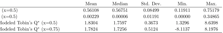
such as effort and expertise.10 Table 2 presents summary statistics forz and y from inverting the
model to actual total assets and CEO pay-performance sensitivity. Considering first CARA with
x=0.5 (Panel A), the mean value ofzis 0.00128, and the median value is 0.00004. The mean value of y is 0.561 and the median value is 0.567. The Pearson (Spearman) correlation between z andy
is -0.107 (-0.523) (p<0.01 (0.01)). The negative correlation betweenzandy is consistent with the previously-documented negative relation between effective CEO ownership (wealth to performance sensitivity) and firm size (e.g., Bizjak, Brickley, and Coles (1993), Schaefer (1998), and Baker and Hall (2004)). In our data, the Pearson (Spearman) correlation between ownership and total assets is -0.108 (-0.556) (p < 0.01 (0.01)). CEOs in larger firms have smaller ownership shares. This is consistent with our model in that idiosyncratic risk (in dollar terms) increases in firm size according toIx.11
Table 2 also reports summary statistics of the modeled values of Tobin’s Q, Q∗, for two values
of the parameter that defines how firm size affects idiosyncratic cash flow risk, x = 0.50, 0.75. With CARA (Panel A) with x = 0.50, the average value of the model-generated Tobin’s Q is Q∗
= 1.83, with a standard deviation of 0.36. When x= 0.75, the average value is Q∗ = 1.86, with a
standard deviation of 0.44. Note that even though our model-generatedQ∗values include a random
disturbance term based on actual cash flow variation, they are still less variable than the actualQ
values observed in the data (Table I). This is not surprising, since actualQis likely to be influenced by additional forces outside of our model. Nonetheless, this comparison of the lower moments of actualQand model-generatedQ∗ suggests that the model represents some of the forces that drive
10The issues in this literature include productivity of inputs (e.g., capital, labor, other materials, and energy),
returns to scale, productivity growth, efficiency of public versus private firms, international comparisons of produc-tivity and efficiency, producproduc-tivity in specific industries (e.g., electric power and agriculture), various functional forms of production functions (Cobb-Douglas, translog, etc.), and the measurement of welfare. The most closely related study to ours we could find is Hellerstein, Neumark, and Troske (1999). This study estimates translog production parameters for four types of workers, and one of those classes contains all professional workers and the management team.
11Again, our model is based on moral hazard, but an alternative would be to focus on adverse selection and sorting
firm structure.
Panel B of Table 2 reports results for approximate CRRA. The moments of Q∗,z, and y are
quite similar to those for CARA. The primary differences are a higher mean and more range in
z and slightly greater range in Q∗. Otherwise, the moments are almost identical between CARA
and approximate CRRA and CRRA Q∗ bears the same relation to actual Qas CARA Q∗. Thus,
hereafter we focus on CARA, though we also continue to provide some results for CRRA where appropriate.
B. Model comparative statics
One significant benefit of fitting a structural model to data is the opportunity to gauge the eco-nomic significance of the underlying structural parameters as determinants of organization form. In our model, the shareholders choose scale of the firm and the managerial compensation scheme (effective ownership) to maximize value. Exogenous variables include scaled margin (p = Ap+), risk aversion (r), unscaled standard deviation (σ), and the scale factor for cash flow risk (x). The parameters governing productivity of managerial input (z) and assets (y) also are exogenous. Ta-ble 3 presents estimates of the effect of each of these parameters on the optimizing choice of size, effective ownership, and model-generated expectedQ in the CARA model. Because δ∗ and I∗ are
highly nonlinear in the structural parameters (see the first-order conditions, (9) and (10)) and, thus, so is EQ∗, we calculate optimal ownership and size for a benchmark level of the parameter
plus and minus a perturbation in that parameter and then calculate the percentage changes inδ∗, I∗, andEQ∗. We perturbp,r,σ,x,z, andy by 10 percent relative to the benchmark levels. In all
calculations, we use p= Ap+ = 40,r = 4, σ = 0.33, and x = 0.50 as the benchmark levels of the
exogenous parameters that do not vary across firms. For the estimated productivity parameters, z
and y, we use the medians (Table 2, Panel A) as benchmark levels.
of managerial input, implies a 4.85 percent change in the optimal effective ownership level of the CEO, all else equal. Accordingly, CEO ownership andz are highly-correlated in the data (Pearson (Spearman) correlation = 0.823 (0.998)). A 10 percent increase iny, which increases the marginal productivity of investment, induces a 4.63 percent decrease in the optimal ownership level of the manager. This effect should be stronger when x is larger because cash flow volatility is more sensitive to scale and compensating the manager for additional risk-bearing is costly. All else equal, a 10 percent increase inz induces a small decrease in firm size and has no discernible effect on EQ∗. In contrast, a 10 percent increase in the value of y induces a very large increase (283.8
percent) in firm size and a 9.13 percent decrease inEQ∗.
Consistent with the operation and basic predictions of our augmented principal-agent model, increases in managerial risk aversion or volatility have a substantial negative effect on the optimal level of CEO ownership. Increases in risk aversion and volatility, however, have only negligible effects on investment and expected Q∗. All else equal, an increase in profit margin, p, increases
the optimal size of the firm, but has negligible effects on ownership andEQ∗. Increasing x, which
determines the extent to which scale affects cash flow volatility, decreases ownership but has very little effect on EQ∗ and scale. When the values of the parameters are decreased by 10 percent
from their benchmark levels, the changes in the endogenous variables have opposite sign and are somewhat different in magnitude, presumably because of the nonlinearities in the model.
5.
Does the Model Conform to Real Data?
The prior section shows that the model survives basic scrutiny on two levels. First, it is invertible for both CARA and approximate CRRA. There always exist productivity parameters for physical assets and managerial input that support observed firm size and CEO pay-performance sensitivity as optimal. Thus, the model satisfies a basic hurdle for validity. Moreover, the lower moments of model-generatedQ∗ (both CARA and CRRA) are similar to those of actualQ. In this section, we
provide more detailed tests of external validity, that is, the ability of the model to conform to real data.
A. Variation across industries
Table 4 reports median values of the estimated structural parameters, z and y, endogenous inside ownership and investment, δ∗ and I∗, and predicted Q (including the random disturbance
term),Q∗, across industries defined following the taxonomy of Fama and French (1997).12 For both
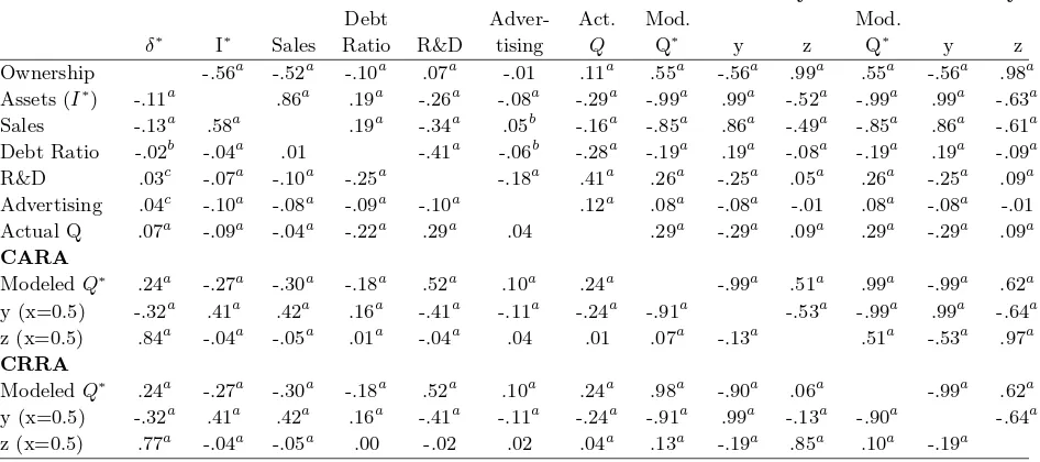
CARA and approximate CRRA, the Pearsonχ2 test of goodness-of-fit rejects the null hypothesis that any ofz,y,z/y,δ∗, and Q∗ do not vary across industries.
A related informal test of our model is whether our estimates of the relative productivity of managerial inputs versus physical capital appear to vary as one might expect across industries. The data in Panel A of Table 4 are sorted by CARAz×104/y. (Note that the ordering of
indus-tries based on CRRA in Panel B differs only slightly.) The ratio z×104/y, a relative measure of the importance of managerial input versus physical capital in the production process, is high in a broad spectrum of industries, ranging from Personal and Business Services (which includes edu-cational services, software development, and networking services), Business Equipment (including computers), Healthcare, and Recreation (which includes the movie industry). The lowest ratios are in industries such as Precious Metals and Metal Mining, Tobacco Products, Utilities
tric, Gas, and Sanitary Services), and Communications. In absolute terms, physical capital is most productive in Financials, Tobacco Products, Aircraft, Ships, and Railroads, Utilities, and Communications, while managerial input is most productive in Personal and Business Services, Restaurants, Healthcare, Business Equipment, and Recreation. Accordingly, median investment is quite large in Tobacco Products, Financials, and Communications, while median managerial own-ership is quite large in Recreation, Healthcare, and Personal and Business Services. These results are consistent with economic intuition about how the productivity of physical and human capital should vary across industries as a function of the technology.
B. Variation within industry
We next examine variation within industry. It is quite plausible that steel companies and service companies have different marginal productivity parameters. But does heterogeneity in those pa-rameters really explain variation in size and contract within the steel and service industries? To address this question, Table 4 reports within industry standard deviations for z,y, andz×104/y. The standard deviation across industries for the average values of z×104, y, and z×104/y are
9.80, 0.035, and 19.97, respectively. In most industries, the within industry standard deviation of the productivity parameters exceeds the cross-industry standard deviation. This suggests that production technology can significantly vary across firms even within the same industry, which is consistent with the large dispersion in firm size and CEO wealth-performance sensitivity within industries observed in the data.
Another interesting question concerning within industry effects relates to the correlation be-tween extracted y and z. Large firms, such as GM, generally have small δ∗, while a small startup
neg-ative correlation in order to fit such data. Largery implies larger size,I∗. Larger I∗ implies larger
idiosyncratic cash flow risk, arising from the disturbance I∗xε˜, which implies lower δ∗. Thus, the
structure of the model does not necessarily require z to be lower when y is higher in order to generate lower δ∗. The data, however, if δ∗ falls substantially in size, may yield such a result. To
examine this further, for each industry we calculate the correlation between z andy. The average within-industry Pearson correlation is -0.18, which is less negative than the cross-industry correla-tion (of means) of -0.25. In order to support observed size and CEO pay-performance sensitivity as optimal choices, the model does not require more negatively correlated productivity parameters within industry than across industries.
A final aspect of variation within industries relates to the possibility that the approximate CRRA formulation is more flexible than the CARA case. The argument is that the CARA model potentially places unreasonable demands on only two parameters,zandy, to explain variation in the data. Certainly it is plausible that the productivity parameters explain variation across industries, but can we really expect the variation of the Cobb-Douglas exponents to explain variation of size and pay-performance sensitivity within each industry? Allowing variation in managerial risk aversion, along with variation in the productivity parameters, may provide more explanatory power, particularly within industries. Thus, we examine whether inverting the CRRA model delivers less variation in the productivity parameters that support δ∗ and I∗ as optimal choices than does
inverting the CARA model. The answer is no. The standard deviation ofy within industry tends to be very similar across the CRRA and CARA formulations. In contrast, CRRA requires more
variation within industry of implied zand z/y than does CARA.
C. Correlation
(R&D intensity, sales, leverage, and advertising effort).
Table 5 provides Pearson and Spearman correlations for the relevant variables. For both CARA and approximate CRRA we report results based on x = 0.5, but the results are similar for other values of x. The Pearson and Spearman correlation coefficients for Q∗ and Q are 0.24 (p < 0.01)
and 0.29 (p <0.01) for both CARA and CRRA. A different incarnation of this same result appears later in Table 8, which presents the results of regressing actual Q on EQ∗ (t = 8.79). It appears
that modeledQ∗ has some power to explain actual Tobin’s Q.
Actual Tobin’s Q is negatively correlated with sales and leverage, and positively correlated with R&D and advertising. Similarly, both CARA and CRRA model-generatedQ∗s display statistically
significant correlations of the same sign with sales leverage, R&D, and advertising.
In sum,Q∗and actualQhave similar lower moments,Q∗has power to explain actualQ, and the
cross moments ofQ∗with variables outside of the model accord well with those same cross moments
of actualQ. These results suggest that the form of our model and the fitted structural parameters capture some of the economic determinants of firm size, CEO pay-performance sensitivity, and firm performance.
6.
Getting Over the Hump: The Relation Between Ownership
and Performance
This section reports results for an important class of tests of external validity. One test examines whether there is a hump-shaped relation betweenQ∗andδ∗. The other examines whether
simple functions ofz and y, the parameters in our model that are purported to determine δ∗, I∗,
A. The link between CEO ownership and firm performance
Consider the often-reported result of an “inverted-U” or “hump-shaped” relation between ownership and Tobin’s Q (e.g., McConnell and Servaes (1990) and Himmelberg, Hubbard and Palia (1999)). One conventional interpretation of this finding is that the incentive effects associated with higher ownership are strong for low to medium levels of ownership, but that entrenchment effects become dominant at high levels of CEO ownership (Stulz (1988)). This explanation requires substantial costs of adjusting managerial ownership. Our alternative is that these results could also arise as the outcome of value-maximizing choices of organizational form driven by underlying features of the contracting environment. The question becomes whether our model can serve to explain the inverted-U. The answer is yes.
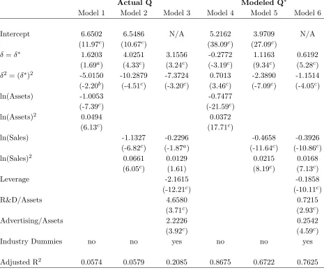
Table VI reports pooled OLS regressions of Tobin’s Q from the actual data and noisyQ∗ from
our model on the ownership share of the CEO (δ) and its squared value. Throughout, all test statistics are adjusted for heteroscedasticity and clustering within firms (per Petersen (2006), see Rogers (1993)). The first model in Table VI reports the results using actual Q as the dependent variable. Consistent with the results reported in many prior studies, our data also reflect the inverse U-shaped relation between Tobin’s Q and ownership. The coefficient estimate on the CEO’s ownership share is 8.61 (t-statistic = 9.00), and the coefficient estimate on the squared ownership of the CEO is -21.46 (t = -8.38). The ratio of the coefficient estimates of the linear term to that of the squared term is -0.40, which corresponds to a maximumQat CEO ownership of 20.09 percent. The adjusted R-squared of the regression is essentially the same as that reported by Himmelberg, Hubbard, and Palia (1999, Table 5) for the same regression specification.
The remaining columns in Table VI present results using as the dependent variable Q∗ values
the coefficients on the linear term to that on the squared term is -0.427, which corresponds to a maximumQ∗ at CEO ownership of 21.34 percent.
Similar results arise in both CRRA models (x = 0.5 in model 4 and x = 0.3 in model 5) and for CARA when we usex = 0.3 (not reported). The estimated relation betweenQ∗ and ownership
is concave, and the level of managerial ownership that defines the top of the hump is similar. Note, however, that the model is capable of delivering a different relation betweenQ∗ and CEO
ownership. Though we focus onx = 0.50, as estimated from our Execucomp firms, the analogous estimate for all firms on Compustat is 0.75. Holding all other parameters in our model constant, this would imply an increasing convex relation betweenQ∗ and CEO ownership, which is not consistent
with the patterns observed in our data. Ownership data on many more firms would be required to examine the shape of the Q-ownership relation for all firms on Compustat. Though our model can give rise to shapes other than the inverted-U, the most natural assumptions for our data (x = 0.5) generate the hump.13 Moreover, if risk aversion is smaller, CARA r = 2 for example, the relation
for x = 0.75 again is concave. In our model, lower x and lowerr tend to favor a concave relation betweenQ∗ and CEO ownership.
B. How the model works
We now explain why the model gives rise to the observed relation between Qand CEO ownership. Consider an increase in the productivity of physical capital, y. As Table 3 indicates, this implies a large increase in investment, a decrease in managerial ownership, and, thus, a decrease in EQ∗
and, consequently, Q∗. On the other hand, Table 3 also shows that an increase in productivity of
managerial input, z, implies an increase in CEO ownership, very little increase in investment (so as to avoid magnifying the exposure of the manager to increased risk), and very little effect onQ∗.
13Variation in empirical findings across studies of theQ-ownership relation could be driven by variation inxacross
Also recall that the estimated productivity parameters, z and y, are negatively correlated in the full sample (Table 5), though the absolute value of that correlation is not particularly large.
Consider first the set of firms for which z and y are negatively related. Increasing z and de-creasingy will lead to an increase in CEO ownership as the effects of increasingzand decreasingy
reinforce each other. In addition, investment (size) declines andQ∗ increases. For firms represented
in this part of the sample,δ∗ andQ∗ will move together. In contrast, consider the subset of sample
firm for which z and y increase together. Referring again to Table 3, the effect on managerial ownership is ambiguous. For large sensitivity of cash flow risk to scale (large x), increasing in-vestment exposes the manager to substantially more risk. This is expensive for the principal, who must compensate the agent (higher α), so optimal managerial ownership falls as the suppressive effect of increasing y on δ∗ more than offsets the effect on δ∗ of increasing z. Q∗ decreases as
well. In this case, once again, δ∗ and Q∗ will move together. On the other hand, for smaller x,
the effect of increasing z dominates the effect of increasing y, so managerial ownership increases on net because increased scale does not unduly expose the manager to higher risk. Thus, size and managerial ownership move together, but Q∗ declines, in which case, for firms in this part of the
sample, increasing δ∗ is associated with decreasing Q∗. It remains to be seen, of course, whether
both of these effects and underlying intuition are reflected in the results from inverting the model. To explicitly examine the above intuition, Table 7 displays median values of the exogenous productivity parameters, endogenous choice variables, and model-generated Q∗, all by observed
CEO ownership deciles. For deciles one through nine, y falls and z increases. Thus, optimal investment falls relative to optimal CEO ownership and, as a consequence, Q∗ increases as the
negative effect on Q∗ of higher y and investment is larger than the positive effect on Q∗ of higher z and managerial input. In this way, the structure of the model and distribution of the exogenous productivity parameters in the data combine to yield a hump-shaped, endogenous relation between
Q∗ and managerial ownership.
C. The power of δ∗ versus the productivity parameters to explain actual Q
Table 8 presents results on the relative power of δ∗ versus EQ∗ and the productivity parameters
to explain performance. For the purposes of comparison, models 5 and 6 present results when the performance measure is Q∗. Relative to model 2 of Table 6, these two regressions illustrate that
including simple transformations of z and y (model 6) or EQ∗ (model 5) usurps the explanatory
power of the quadratic in CEO ownership. Of course, this exercise is rigged. Notwithstanding the overly simple functional forms ofz and y, it would be quite surprising if the results were different. After all, the exogenous productivity parameters and the model determine the endogenous variables
Q∗, δ∗, and I∗. In contrast, in no way was construction of the model and estimation of the
productivity parameters informed by matching the model to data on actual Q. Thus, the real question is whether the same results arise when we go outside the model to consider Qcalculated from Compustat data.
The benchmark for comparison is Model 1 of Table 6, which represents how the hump-shaped relation between actualQ and CEO ownership appears in our data. The estimated coefficients are 8.61 on δ∗ (t = 9.00) and -21.46 on the square of δ∗ (t = -8.38). The question is whether EQ∗ or
the productivity coefficients diminish the explanatory power ofδ∗ and its square in the regression.
As model 2 indicates, however, including model-generated EQ∗ instead ofzandy on the
right-hand side does not render the ownership variables insignificant, although the magnitudes of the coefficient estimates decline substantially compared to those reported for Model 1 in Table 6. Thus, despite the empirical success of our approach, it is doubtful that our model encompasses all of the relevant economic determinants of firm size and managerial ownership. Perhaps no parsimonious model can. Nonetheless, our simple model does provide substantial explanatory power. We discuss this further in subsection VI.E.
D. Additional analysis
Many studies on ownership and performance use a broader measure of managerial ownership (e.g., the total ownership of all officers and directors reported in the proxy statement). Thus, we repeat the analysis using our ownership measure aggregated over the top executive group as specified in Execucomp. The results are very similar. In our sample, top executive ownership averages 0.049 and varies from less than 0.001 to 0.810. The ownership of top executives is highly correlated with CEO ownership (Pearson correlation = 0.865, p-value < 0.01). Accordingly, it is not surprising that the results using top-executive ownership are very similar to those reported above based on CEO ownership. For x = 0.50, the mean values of the calibrated productivity parameters y and
z are 0.563 and 0.002, respectively. The tests on lower moments, industry, and correlations all yield similar results. Regressing modeled Q∗ on total executive ownership yields coefficients on
ownership and ownership squared of 3.882 (p< 0.01) and -6.758 (p<0.01), respectively. By way of comparison (to McConnell and Servaes (1990)), regressing actual Q on the broad measure of ownership and its squared value yields coefficient estimates of 7.745 (p < 0.01) and -15.687 (p <
0.01), respectively. Repeating the analysis in reported in Table 8, we again find that the extracted productivity parameters usurp the power of δ and its square to explainQ∗ and Q.
to suffer from measurement error in the time series. By inverting the model, this measurement error will be transferred to the calculated values of the productivity parameters y and z. To attempt to minimize measurement error we calculate the time-series average of CEO ownership and firm size for each firm in the sample and then invert the model, as before, to obtain a cross-section of parameters, z and y. The results, which come purely from the cross section of firms, are very similar to those we report and are consistent with reduced measurement error in ownership and assets. For x= 0.50, the mean values of the calibrated productivity parameters y and zare 0.561 and 0.001, respectively. Regressing modeled Q∗ on average ownership yields coefficients on CEO
ownership and ownership squared of 5.099 (p<0.01) and -14.246 (p<0.01), respectively. By way of comparison, regressing the time-series average of actual Q on the time-series average value of ownership and its squared value yields coefficient estimates of 9.872 (p < 0.01) and -26.505 (p <
0.01), respectively. Based on time-series averages, simple functions of average z and y eliminate the power of averageδ andδ2 to explain averageQ∗ and Q.
Our modified-calibration approach calculates the pair (zjt, yjt) that Solves the first-order
condi-tionsSδ(δjt, Ijt, zjt, yjt, x, r, σ2, p) = 0 and SI(δjt, Ijt, zjt, yjt, x, r, σ2, p) = 0, for firms j = 1,2, . . . ,
J and time t = 1,2, . . . ,T (while assuring a global maximum). Other more traditional methods could be employed. For example, we could assume that the productivity parameters are the same for all firms within an industry through time. One could then apply GMM or MLE to observations on (δjt, Ijt), for firmsj = 1,2, . . . , J and timet = 1,2, . . . ,T, to estimate (zk, yk) for industriesk
= 1,2, . . . ,K. We do so and find cross-industry variation in productivity parameters much like that presented in Table 4.
phenomena represented by our model do a good job explaining variation of size and contract form both across and within industries.14
E. Further discussion
Based on both informal and formal comparisons with the data, our model of the performance-ownership relation appears to be empirically successful and, we would argue, conceptually successful as well. Nonetheless, there are opportunities for improvement and further work.
One observation is that the model itself generates a linear contract. But we include options when we estimate effective CEO ownership. This is an inconsistency in application of the model to data, but we believe the model to be a reasonable first approximation. A second-generation model would generate a mix of stock and options as an optimal solution to the contracting problem (see, for example, Lambert and Larcker (2004)). Such a model could treat the incentives to alter the riskiness of investment policy and financial policy (see Coles, Daniel, and Naveen (2006)). Potential approaches to fitting such a model to the data include the one presented herein, as well as standard estimation methods.
Ownership by outside shareholders is the obverse of managerial ownership, so illuminating the determinants of one reveals some of the determinants of the other. Thus, our approach and results are likely to be relevant for recent work on why and how U.S. firms become more widely held after IPO (e.g., Helwege, Pirinsky, and Stulz (2005), Mikkelson, Partch, and Shah (1997)). For future work we leave both the application of a structural approach to that issue and further exploration of whether the specific model in this paper explains outside ownership.
14Another approach that allows both within- and cross-industry variation and familiar types of statistical tests is
simulated method of moments. The procedure is to impose a probability distribution on (x, r, σ2, p) draw repeatedly
from that distribution (N times), and invert the model to retrieve (z, y) for each draw for (δ, I), and then repeat the same process for each and every remaining firm-year observation on (δjt, Ijt). This would yield N (not just 1)
As Table 8 demonstrates, despite the empirical success of our approach, it is doubtful that our model encompasses all of the relevant economic determinants of firm size and managerial ownership.15 We do not suggest, however, that these and other forces are unimportant. There is
plenty of evidence in the literature, as well as in our own empirical analysis, to suggest they are. It is quite likely that factors other those represented inEQ∗ (model 2), other even than z and y,
affect managerial ownership, investment, and firm size. Such variables include the mechanics of stock and option accumulation by managers through the managerial life cycle, factor (e.g., energy) prices, takeovers, exchange rates, monetary and fiscal policy, government regulation, tax law, the marginal tax rate, and exchange rates. Our model can be nested within a model that includes additional such factors, in which case formal statistical tests of their explanatory power would be simple to perform. This is a logical next step.
Along similar lines, we do not provide a formal test of our model versus any of the existing stylized models, such as that of Stulz (1988). Such a test would require nesting entrenchment, perquisite-taking, or other forces in the model. For example, one model might build on ours to include a parameter representing managerial preference for size. One possibility is that managers have a positive preference for span of control or size. The other possibility is that managers prefer smaller firms, a preference that could be driven by risk avoidance. After calculating the relevant parameter for each firm (manager)-year observation, standard methods would test for whether the average manager has any preference for size and whether that preference differs across managers as a function of proxies for the level of managerial entrenchment. We leave this for future work. For the time being, our analysis does illustrate the difficulty of discriminating among alternative interpretations in the absence of a well-specified model of firm behavior. Furthermore, our analysis demonstrates the opportunities for doing so in a model such as ours.
7.
Econometric Approaches to the Endogeneity Problem
In empirical corporate finance, many inferences are based on estimated coefficients from reduced-form regressions of either performance on structure or of structure on other structure variables. Structural dimensions of particular interest include managerial compensation, board composition, board size, ownership structure, debt policy, investment policy, dividend policy, lead-ership structure, antitakeover protections, and product market strategy. Performance measures include accounting profit, stock returns, debt returns, and Tobin’s Q. Most studies mention the possibility of endogeneity, and a good number implement standard econometric approaches, such as fixed effects and simultaneous equations methods.
It is possible that the endogeneity problem in practice has little economic or statistical impor-tance, because either reduced-form OLS regression methods are appropriate or implementing the standard econometric antidotes is effective. The alternative, which is less appealing, is that some results are driven by omission of some important aspect of the environment that determines both the dependent and independent variables together, in which case the results reveal little about cau-sation or the underlying structure of the economic problems organizational choices are purported to solve. Himmelberg (2002), which provides a clear and persuasive discussion of this issue, notes that this complaint applies with equal force to regressions of either performance or governance features on other governance features.
So our purpose, in this section, is to assess the empirical importance in corporate finance of the endogeneity problem. The opportunity to do so arises because we specify and fit a structural model to the data. Of course, based on the model “calibration,” managerial ownership and total assets from the model perfectly match those in the sample of actual firms. So we turn the model around. We assume the model and productivity parameters are correct and then use the model to generate simulated data, specifically endogenously-determined Q∗. In essence, we create a data
Regardless of whether one believes our model is theright model, this approach provides a relatively clean framework for evaluating the severity of the endogeneity problem.
A. When we know the model
Knowing the model, as we do, provides a convenient point of departure. Even after adding a scaled, randomly-generated disturbance term, we should be able to fit Q∗ to the underlying, structural
parameters, so long as we include all relevant exogenous variables in the correct functional form. Based on the results in model 4-6 of Table 8, we already know this works. Including EQ∗, which
encompasses the productivity parameters, optimal choice of ownership and size, and the correct formulation forQ, provides explanatory power forQ∗ (model 4) and also appropriates power from
the quadratic inδ∗ (model 5). Of course, it is possible that the researcher does not know the exact
functional form to use for the exogenous parameters. Thus, model 6 uses a relatively simple set of nonlinear functions ofzandy to control for the structural determinants ofQ∗(andδ∗ andI∗). The
approximation does a very good job of explaining variation in model-generated Q, the estimated parameters onδ∗andδ∗2are insignificant and small, andδ∗ andδ∗2 together have little explanatory
power. In our simulated data, including the exogenous variables in the regression eliminates the “spurious” relation between two endogenous variables. Effort directed toward identifying such variables and collecting the relevant data is likely to be worthwhile.
B. Instruments for omitted variables
Inverting the model yields estimates of bothz and y for each firm-year observation in the sample. But, in general,zandy(as well asp,r,σ, andx) are not observable to the econometrician, though the parameters will be correlated with the endogenous choices, δ∗ and I∗, and performance, Q∗.
most common of these is some measure of firm size (e.g., Morck, Shleifer, and Vishny (1988), McConnell and Servaes (1990), and Himmelberg, Hubbard, and Palia (1999)). The idea is that if CEOs generally own smaller stakes in large firms and if Q is negatively correlated with firm size, then omitting firm size from the regressions will lead to a spurious positive relation between CEO ownership and Q.
To investigate this issue, Table 9 presents results from misspecified (excluding z, y, EQ∗)
regressions of both actual and modeled Q values on CEO ownership, squared CEO ownership, measures of firm size, and additional control variables used elsewhere in the literature. The primary tests are those that take place entirely within the model, with Q∗ (x = 0.50) as the dependent
variable (models 4-6), but for comparison purposes we also estimate the same specifications with actualQon the left-hand side (models 1-3). To measure firm size, we follow Himmelberg, Hubbard, and Palia (1999) and include the natural log of assets (sales) and its squared value. Note that, in our model, total assets also is endogenously determined. Thus, we use the natural log of sales as an alternative instrument. In some specifications we also include leverage, the ratio of R&D expense to total assets, the ratio of advertising expense to total assets, and indicator variables for each two-digit industry in the sample.
Consider the three specifications based onQ∗. When book assets is used to measure firm size, the
coefficients on the ownership variables change sign from their values in the corresponding regressions reported in Table 6. The coefficient on CEO ownership becomes negative and the coefficient on the squared term becomes positive. Both coefficients are significant at the 1 percent level. In this case, we know that firm size is endogenously determined along with Q∗ and ownership, and thus
the dramatic change in the coefficient must be the result of model misspecification.16 In particular,
the results suggest that the relation between the endogenous variables is non-linear. In contrast, when sales is used to measure firm size, the coefficients on CEO ownership and squared ownership
16Parameter estimates from ordinary least squares regressions will be biased when the regressors are endogenously
retain their signs from the regressions in Table 6 (model 2), although the absolute magnitudes of the coefficient estimates are reduced by about half. Nevertheless, the coefficient estimates on both variables remain statistically significant at the 1 percent level. Finally, model 6 shows that adding standard control variables does not usurp the explanatory power of the ownership variables, both of which remain statistically significant at the 1 percent level.
The results are quite similar when we depart from simulated data to employ actual Q as the dependent variable. Using book assets (model 1) as a control, the coefficients on both CEO own-ership and the squared ownown-ership variable are reduced in absolute magnitude compared to model 1 of Table 6. The linear term remains statistically significant at the 10 percent level (t = 1.69) and the squared term is significant at 5 percent (t = -2.20). Actual Q is significantly negatively related to the log of assets, and the relationship is convex as the coefficient estimate on the squared term is positive. When sales is used to measure firm size, the coefficients on CEO ownership and the squared ownership variables are closer to the values from the benchmark regressions (Table 6, model 1). Moreover, both coefficients are significant at the 1 percent level. Adding leverage, R&D, advertising, and dummy variables to control for industry effects does not eliminate the explanatory power of the ownership variables. The hump-shaped relation remains and the estimated coefficients on both ownership and ownership squared continue to be both large and statistically-significant at the 1 percent level.
and from the fact that the relationship between Tobin’s Q and ownership is driven by a nonlinear function of these exogenous variables.
C. Fixed effects and unobserved firm heterogeneity
Himmelberg, Hubbard and Palia (1999) suggest using firm fixed-effects to control for unobserved heterogeneity in the contracting environment (e.g., differences in managerial quality). This pro-cedure relies on time-series variation alone to identify the relation between firm performance and ownership. In this subsection, we examine the use of firm fixed effects to control for unobserved firm heterogeneity in our model-generated data. Since we match the model to observed values of ownership and book assets in each firm and year, our model-generated data contain any firm-specific attributes associated with the contracting environment that do not vary (or vary only slightly across time).
We follow Himmelberg, Hubbard, and Palia (1999) and include only firms with three years or more of data in our panel. This creates a panel of data consisting of 7,562 firm-year observations from 1,458 different firms. The last four columns in Table 10 use modeled Q∗ as the dependent