A new Test of Uncovered Interest Rate Parity: Evidence from Turkey

(1)

Munich Personal RePEc Archive

A new Test of Uncovered Interest Rate

Parity: Evidence from Turkey

Erdemlioglu, Deniz M

Bogazici University, Department of Economics - ECONFIN

August 2007

Online at

https://mpra.ub.uni-muenchen.de/10787/

(2)

A new Test of Uncovered Interest Rate Parity:

Evidence from Turkey

Deniz Erdemlioglu1_{, Bogazici University, Istanbul}

Prof. Dr. C. Emre Alper, Bogazici University, Istanbul, Adviser

Department of Economics Bogazici University

August 2007

Abstract

This paper examines if uncovered interest rate parity condition holds for Turkey. In this paper, an empirical analysis is provided for the dates between December 2001 and June 2007 by using monthly data for Turkey and the U.S. Main finding is that UIP does not hold for Turkey. In addition to this, UIP deviation goes up over time, AR (1) fits the data well, there is an ARCH effect and GARCH (1,1) specification is significant for Turkish case.

Keywords: Uncovered Interest Rate Parity, Unit Root Test, AR Process, ARCH and GARCH Models.

Correspondence: Catholic University of Leuven, Belgium. Email: deniz.erdemlioglu@student.kuleuven.be

1

Predoctoral Research Student (M.A.S.E), Department of Economics, Catholic University of Leuven, Belgium. This paper has been written as a Masters Project of Economics and Finance Program at Bogazici University. I am thankful to Professor C. Emre Alper for his helpful comments and suggestions in writing this paper. All errors are mine.

(3)

1. INTRODUCTION

Uncovered interest rate parity (UIP) states that the nominal interest rate differential

between two countries must be equal to expected change in the exchange rate. In other words,

if UIP condition holds, then high yield currencies should be expected to depreciate. Thus, any

finding reflecting exchange rate appreciation rather than depreciation is called Forward

Premium Puzzle. UIP also postulates that, if covered interest rate parity holds, then the interest

rate differential is an unbiased predictor of the ex post change in the spot exchange rate,

assuming rational expectations (Chinn, 2007). This is called unbiasedness hypothesis in the

UIP literature.

The fundamental assumption underlying UIP is the Efficient Market Hypothesis.

Obviously, the EMH tells us the price should fully reflect all the information available to the

market participants and hence no excess return will be possible in the market. Moreover, EMH

can be considered as a joint hypothesis that market participants have rational expectations and

that they are risk neutral (Taylor, 1995). If these assumptions are valid and UIP holds then the

expected return from holding one currency rather than another is offset by the opportunity cost

of holding funds in that currency versus another (Foy, 2005).

This paper is organized as follows. In the next section, we examine the theory behind

UIP and look at the existing literature regarding the conventional empirical studies used to test

UIP. In section 3, we describe the data set and sources. Section 4 contains an empirical work in

(4)

2. THEORY

UIP can be derived by using CIP, unbiasedness hypothesis, rational expectations and

risk-neutrality assumptions. As long as no arbitrage opportunity exists, the forward discount –

the difference between forward rate and spot exchange rate at time t – will be equal to the

interest rate differential between two countries:

* )

(

t t t k

t

s

i

f







₍₁₎

where ft(k)is the logarithm of forward exchange rate for maturity k periods ahead, stis the

logarithm of spot exchange rate at time t, i_t is the k-period yield on the domestic instrument,

and it* is the corresponding yield on the foreign instrument. Note that equation (1) is also called

covered interest rate parity (CIP).

Equation (1) holds regardless of investor preferences. However, if the investors or

market participants are risk-averse, then the forward rate will differ from the expected future

spot exchange rate by a premium that compensates for the perceived riskiness of holding

domestic versus foreign assets (Chinn, 2006). Thus, the risk premium,, is defined as:

1 1

) (





_t _t _t

k

t

E

s

f



(2)

Assuming CIP holds, substitute Eq. (2) into Eq. (1):

* 1

1 t t t t

t

s

i

E

_





_







(3)

Rearranging Eq. (3) gives:

1 *

1 





t



t



t



t

s

i

E



(4)

Recall UIP is based on the joint hypothesis that market participants have rational expectations

and that they are risk-neutral. Therefore, the rational expectations assumption can be defined

(5)

1 1

1  





t t



t t

E

s



(5)

where s_t_₁ is the logarithm of future spot exchange rate, E_tS_t_₁ is the expectations of spot

exchange rate at time tconditional upon information available at time t, and t_₁ is the rational

expectations forecasting error realized at time t + 1 from a forecast of the exchange rate made

at time t. Now, substituting Eq. (5) into Eq. (4) will enable us to apply rational expectations

assumption into UIP condition:

1 1

*

1  





t



t



t



t



t t

s

i

s





(6)

Furthermore, applying the other crucial assumption, risk-neutral behavior, _t_₁ 0 gives UIP

relationship:

1 *

1 





t



t



t



t

s

i

s



(7)

In order to test Eq. (7), UIP, the following regression model will be estimated,

1 *

1

(

)













s

_t





i

_t

i

_t



_t (8)

where st_₁ denotes the change in the exchange rate in logarithms,  and  are the regression

coefficients, (i_t i_t*) denotes the interest rate differential, and _t_₁ is the forecasting error

realized at time t +1 from a forecast of the exchange rate made at time t.

The last equation is the conventional UIP regression which has been used to test UIP in

the literature. The null hypothesis of UIP can be expressed as Ho:=0, =1, but in fact, the

literature usually focus on the slope coefficient,2.

The null of unity, =1, has been mostly rejected in the literature. Isard (2006) found

that the estimated intercept and the slope coefficient in equation (8) are significantly different

from zero and one respectively for less than 1 year horizon. Similarly, Foy (2006) estimates

equation 8 by using OLS and rejects the null of unity. He also finds that the estimated slope

2

(6)

coefficient is less than one and also negative. This finding also reflects the existence of

Forward Premium Puzzle indicating higher interest rate currency continues to appreciate, not

depreciate. Bruggemann and Lutkepohl (2005) conduct an empirical study based on unit root

test and univariate analysis for the monthly market and 10 year bond rate for the period

1985-2004. They show evidence3 of EMH and UIP to hold jointly for the U.S. and Europe. Meredith

and Chinn (2002) test unbiasedness hypothesis as well as UIP. Their short horizon study4

indicates that the unbiasedness hypothesis does not hold and UIP condition fails over short

horizon. On the other hand, they find correct sign and hence do not reject the null of unity over

long horizons. Kool (2006) also estimates the equation 8. His results are consistent with those

of Foy (2006). Kool (2006) found that the estimated slope coefficient is negative for each of

the ten countries. Flood and Rose (1997) argues that whether or not UIP holds depends on the

exchange rate regime. For this aim, they perform an empirical study5 by estimating the same

conventional equation and conclude that UIP does not hold. Moreover, forward discount puzzle

vanishes for fixed exchange rates. Chinn (2006) examines UIP and unbiasedness hypothesis

over both short and long horizons. His empirical results suggest that the unbiasedness

hypothesis as well as UIP appear to work much better over long horizon indicating zero

intercept and unity cannot be rejected6. On the other hand, Chaboud and Wright (2003) perform

a high frequency data7 study. By using ordinary UIP regression, equation 8, they could not find

evidence to reject unity for shorter horizons. Flood and Rose (2002) found an interesting result

that UIP works systematically worse for fixed and flexible exchange rate countries than for

3

B&L’ s robustness check including multivariate analysis, cointegration analysis within VECM provides similar results in their paper.

4

Quarterly data, 3-6-12 month movements in the exchange rates, and GMM estimators for the econometric analysis. Long horizon analysis is conducted for 5 year yields for Germany, UK and Canada.

5

Flood and Rose (1997) use “seemingly unrelated regression technique” and Newey-West estimators in their econometric study.

6

See Isard (2006) for similar results in long horizon case.

7

(7)

crisis. The empirical results of Bekaert, Wei and Xing (2005)8 present that UIP depends on the

currency pair, not horizon. Furthermore, a random walk model for both interest rates and

exchange rates fits the data marginally better than UIP model9.

Obviously, the papers discussed above shed light on issues of data frequency, horizon

selection, null of unity, forward premium puzzle and unbiasedness property. Therefore, the vast

evidence for rejection of UIP makes researchers examine the joint assumption of rational

expectations and risk-neutrality. For instance, Taylor (1995) and Isard (2006) confirm that

possible explanations of rejecting UIP are based on rational expectations and/or risk neutrality

assumptions, peso problem, self-fulfilling prophecies, rational learning under incomplete

information and simultaneity bias10. The most common literature solutions for violation of joint

hypothesis are using survey data for rational expectations and modeling risk premium for risk

neutrality assumption11. In addition to these explanations, Marey (2004) takes rational

expectations assumption seriously and concludes that different expectation models induce

different slope coefficients embedded equation 8. Eventually, Chakraborty (2007) generates a

monetary model with bounded rational agents who are learning and updating their knowledge.

He finds that the estimated negative slope coefficient which has received so much attention in

the literature is a reflection of learning dynamics.

8

In this econometric study, Bekaert, Wei and Xing (2005) use VAR tests, implied VAR statistics, Monte Carlo Analysis, LM and Distance Metric Tests.

9

See also Thornton (2007) for similar conclusion.

10

See Taylor (1995) for rational expectations and risk neutrality criticization,; Flood and Rose (1997) for peso problem.

11

(8)

3. DATA

The data set consists of monthly observations of YTL/USD exchange rate, as well as

domestic and foreign interest rates for Turkey and the United States for the period 2001:12 –

2007:06. The interest rate and exchange rate data are constructed from two sources. The

exchange rate data has been obtained from the Central Bank of Turkey (CBRT) and the last

observations of each month have been used in the exchange rate data set in the econometric

study. The domestic interest rate data is overnight interest rate data of the CBRT obtained from

its simple interest rate weighted average category under interbank money market transaction

summary. The original data is daily and hence has been converted to monthly observations

discarding weekends. For the U.S. foreign interest rate data, we used monthly fed funds rate

obtained from Federal Reserve Economic Data (FRED II). Also note that both domestic and

foreign interest rates are simple annualized interest rates. Therefore, we have compounded

annual rates to monthly rates. The plots of the foreign interest rate, domestic interest rate and

spot exchange rate series are provided in appendix.

4. EVIDENCE

This empirical study comprises of three main steps. In the first part, we are going to

look UIP deviation and run the conventional UIP regression in order to test if UIP holds for

Turkey. In the second step of the study, the objective is to find a model for UIP deviation. In

the third step, whether or not a volatility model may explain the UIP deviation will be

discussed.

UIP deviation is basically the difference between the depreciation rate (change in the

spot exchange rate) and the interest rate differential. In that sense, any deviation from UIP

(9)

Figure 1UIP deviation for the period 2002:01- 2007:06

Figure-1 illustrates the UIP deviation in Turkey from January 2002 to June 2007. As

this figure shows, UIP deviates and goes up from 2002 to mid-2006. After that time, UIP

deviation is a bit stable around the level -1’s.

Figure 2 Scatter diagram of interest rate dif. and depr. rate

Figure-2 shows that there is no clear relationship between the interest rate differential

and the depreciation rate. However, a regression analysis may provide a better explanation to

understand if UIP holds.

-5 -4 -3 -2 -1 0

2002 2003 2004 2005 2006 2007 DEVIATION

0.00 0.01 0.02 0.03 0.04 0.05

-0.2 -0.1 0.0 0.1 0.2

(10)

Table-412 shows the regression results of the estimated conventional UIP model13.

Recall that the null hypothesis for testing UIP is Ho: =0, =1. As we look at our regression

results, the estimated regression coefficients are -0.0010 and -0.0015 with the probabilities of

0.91 and 0.99, respectively. Therefore, the null of zero intercept cannot be rejected at 1%, 5%

and 10% significance level. Moreover, there is no evidence that the estimated slope coefficient

is statistically different from zero at all 1%, 5% and 10% significance levels. An extremely low

R-square, 0.000000 also suggests that variation in the interest rate differential cannot explain

the variation in the depreciation rate. These results indicate that UIP does not hold for Turkey.

In other words, the interest rate differential between Turkey and the U.S. is not able to explain

the change in the YTL/USD spot exchange rate for the period 2001:12 – 2007:06.

Table-2 and Table-3 represent Augmented Dickey-Fuller Unit Root Tests on the interest

rate differential and the spot exchange rate respectively. As Table-2 indicates if we test for unit

root in 1st difference including intercept in the test equation, the ADF test statistics will be

more negative than MacKinnon critical values at 5% and 10% significance level. Thus, interest

rate differential is I(1)14. Moreover, testing for unit root in 1st difference including intercept in

test equation suggests that the spot exchange rate is also I(1). In fact, these results are

consistent with the UIP literature.

Having seen the rejection of UIP based on regression analysis by using OLS, now, we

are going to look for alternative models of UIP deviation. The Table-6 provides the

correlogram Q-statistics test for residuals obtained from the regression of UIP deviation on the

constant term. This table illustrates that the p-values are closed to zero and hence the null of no

autocorrelation can be rejected at 1%, 5% and 10% significance level. This means that there is

an autocorrelation problem between the residuals. Moreover, since the residuals are

12

All Tables are provided in appendix.

13

All series are assumed I(0) in this step. The stationarity of the series as well as unit root tests will be discussed later.

14

(11)

autocorrelated as a result of regressing UIP deviation on constant term, AR(1) model can also

be estimated in order to see if autocorrelation problem is eliminated. Table-7 illustrates ACF

and PCF of AR(1) and it can be seen that the null hypothesis of no autocorrelation cannot be

rejected at 1% and 5% significance level for the residuals of the AR(1) model. Furthermore,

Table-8 provides the estimation output of AR(1) model and suggests that AR(1) fits the data

well.

The last step in the empirical part is to examine ARCH and GARCH-type process for

UIP deviation. Obviously, the reason to examine ARCH effect as well as GARCH specification

is for considering the possible effect of volatility of UIP deviation. In order to do that, first

ARCH effect has been tested for AR(1) model of UIP deviation. Then, ARCH and GARCH

models have been estimated by using ML - ARCH methodology.

Table-9 presents ARCH effect test results. According to the table, the probability of

F-statistics is about 0.03 and hence indicates that the null of no ARCH effect can be rejected at

5% and 10% significance level. This result shows that there is an ARCH effect for UIP

deviation based on our data set. Furthermore, Table-10 illustrates both estimated ARCH and

GARCH specifications. It is obvious that the coefficient of GARCH(1) specification in the

variance equation is statistically significant at 5% and 10% significance level. Furthermore, the

estimated slope coefficient of AR(1) is statistically significant at 1%, 5% and 10% significance

level. Table-10 also reflects that the estimated slope coefficient of ARCH(1) specification in

the variance equation is significant at 10% significance level. As a result, we have found the

evidence of both significant ARCH effect and significant GARCH specification for the UIP

deviation.

(12)

5. CONCLUSION

The vast literature shows that Uncovered Interest Rate Parity (UIP) fails empirically.

The reasons for rejection of UIP might be the violation of the joint hypothesis of rational

expectations and/or risk- neutrality. Moreover, empirical studies confirm that peso problem,

self-fulfilling prophecies, rational learning under incomplete information and simultaneity bias

might be the other reasons to reject UIP. In this paper, first, we tested UIP for Turkish case by

estimating the conventional UIP regression. Then, the effect of volatility of UIP deviation has

been examined in the empirical part of the study. Our results indicate that UIP does not hold for

Turkey for the dates between December 2001 and June 2007. Moreover, AR(1) model of UIP

deviation fits the data well, there is an ARCH effect, and GARCH specification is significant

for the UIP deviation in Turkey. Further studies focusing UIP relation as well as deviation may

(13)

References

Ballie, R.T., Bollerslev, T. (2000). “The Forward Premium Anomaly is not as Bad as You Think”, Journal of International Money and Finance, 19 (2000), pp. 471-488.

Bekaert G., Wei M., Xing Y. (2005). “Uncovered Interest Rate Parity and the Term Structure”,

Elseiver Science (preprint), (11 May 2005), pp. 1-70.

Brooks, C. (2002). “Univariate Time Series Modeling”, Introductory Econometrics for

Finance, (Cambridge: Cambridge University Press).

Brooks, C. (2002). “Modeling Volatility and Correlation”, Introductory Econometrics for

Finance,(Cambridge: Cambridge University Press).

Bruggemann, R. and Lutkepohl, H. (2005). “Uncovered Interest Rate Parity and the Expectations Hypothesis of the Term Structure: Empirical Results for the U.S. and Europe”, SFB 649 Discussion Paper 2005-035, (April 4, 2005), pp. 1-16.

Chaboud Alain P., Wright Jonathan H. (2003). “Uncovered Interest Rate Parity: It Works, but not for Long”, FED Paper, (May 2003), pp. 1-30.

Chakraborty, A. (2007). “Learning, the Forward Premium Puzzle and Market Efficiency”,

Department of Economics, University of Tennessee, 506 Stokely Management Center,

(January 24, 2007), pp.1-34.

Chinn, M. (2007). “Forward Premium Puzzle”, World Economy – Forward Premium Puzzle1

(entry written for the Princeton Encyclopedia of the World Economy), (2007), pp. 1-8.

Chinn, Menzie D. (2006). “The (Partial) Rehabilitation of Interest Rate Parity in the Floating

Rate Era: Longer Horizons, Alternative Expectations, and Emerging Markets”, Journal

of International Money and Finance, 25 (2006), pp. 7-21.

Chinn, Menzie D. and Meredith, G. (2002). “Testing Uncovered Interest Parity at Short and

Long Horizons during the Post-Bretton Woods Era”, JEL Classification No: F21, F31,

F41, (June 10, 2002), pp.1-32.

Chinn, Menzie D. and Meredith, G. (1998). “Long-Horizon Uncovered Interest Rate Parity”,

NBER Working Paper Series, Working Paper 6797, (November 1998), pp.1-34.

Engel, C. (1995). “The Forward Discount Anomaly and the Risk Premium: A Survey of Recent

Evidence”, NBER Working Paper Series, Working paper 5312 (1995), pp. 1-117.

Espinosa, Sonia P. (2002). “Testing Uncovered Interest Rate Parity: The Spanish Case”,

FEDEA, EEE 128, (April 2002), pp.1-35.

Flood, Robert P. and Rose, Andrew K. (2002). “Uncovered Interest Parity in Crisis”, IMF Staff

(14)

Flood, Robert P. and Rose, Andrew K. (1997). “Fixes: Of the Forward Discount Puzzle”, IMF

research Department, JEL Classification No: F31, ( May 23, 1997), pp. 1-13.

Foy, Teresa M. (2005). “An Empirical Analysis of Uncovered Interest Rate Parity and the

Forward Discount Anomaly”, Department of Economics, Queen’s University, Ontario,

Canada, K7L 3N6, (March 29, 2005), pp.1-8.

Harvey, John T. (2006). “Modeling Interest Rate Parity: A System Dynamics Approach”,

(Presented at the Association for Evolutionary Economics Conference), (January 2006),

pp. 1-14.

Harvey, John T. (2004). “Deviations from Uncovered Interest Rate Parity: A post Keynesian Explanation”, Journal of Post Keynesian Economics, (2004), pp. 1-28.

Isard, P. (2006). “Uncovered Interest Parity”, IMF Working Paper, IMF Institute, (April 2006), pp. 1-12.

Kool, C. and Hadzi-Vaskov, M. (2006). “The Importance of Interest Rate Volatility in Empirical Tests of Uncovered Interest Parity”, Tjalling C. Koopmans Research

Institute, Discussion Paper Series 06-16, (October 2006), pp. 3-37.

Lothian James R., Wu L. (2005). “Uncovered Interest Rate-Parity over the Past Two Centuries”, Seminar Paper, Center for Research in International Finance at Fordham

University, (June 18, 2005), pp. 1-47.

Marey, Philip S. (2004). “Uncovered Interest Parity Tests and Exchange Rate Expectations”,

ROA, Maastricht University, (March, 9 2004), pp.1-25.

Mccallum, Bennett T. (1992). “A Reconsideration of the Uncovered Interest Parity Relationship”, NBER Working Papers Series, Working Paper No: 4113, (July 1992), pp. 1-43.

Taylor, M. P. (1995). “The Economics of Exchange Rates”, Journal of Economic Literature, 33, pp. 13-47.

Teng, Y. (2006). “An Introduction to Covered and Uncovered Interest Parity”, Economics 826,

Queen’s University, Kingston, Ontario, Canada, (January 22, 2006), pp.1-6.

Thornton, Daniel L. (2007). “Resolving the Unbiasedness and Forward Premium Puzzles”,

Working Paper 2007-014A, Research Division, Federal Reserve Bank of St. Louis,

(15)

Appendix

OBS SPOT RTR RUS

2001:12 1.44 4.92 0.15

2002:01 1.32 4.92 0.14

2002:02 1.40 4.88 0.15

2002:03 1.33 4.61 0.14

2002:04 1.33 4.29 0.15

2002:05 1.41 4.00 0.15

2002:06 1.60 4.00 0.15

2002:07 1.68 4.00 0.14

2002:08 1.63 3.84 0.15

2002:09 1.65 3.83 0.15

2002:10 1.67 3.83 0.15

2002:11 1.54 3.71 0.11

2002:12 1.64 3.67 0.10

2003:01 1.65 3.67 0.10

2003:02 1.61 3.67 0.11

2003:03 1.71 3.67 0.10

2003:04 1.59 3.63 0.11

2003:05 1.44 3.42 0.11

2003:06 1.43 3.19 0.10

2003:07 1.43 3.04 0.08

2003:08 1.40 2.71 0.09

2003:09 1.38 2.56 0.08

2003:10 1.49 2.28 0.08

2003:11 1.47 2.17 0.08

2003:12 1.40 2.17 0.08

2004:01 1.34 2.17 0.08

2004:02 1.33 2.00 0.08

2004:03 1.31 1.92 0.08

2004:04 1.44 1.83 0.08

2004:05 1.49 1.83 0.08

2004:06 1.49 1.83 0.09

2004:07 1.47 1.83 0.11

2004:08 1.50 1.83 0.12

2004:09 1.50 1.71 0.13

2004:10 1.47 1.67 0.15

2004:11 1.42 1.67 0.16

2004:12 1.35 1.59 0.18

2005:01 1.33 1.44 0.19

2005:02 1.29 1.39 0.21

2005:03 1.37 1.32 0.22

2005:04 1.38 1.26 0.23

2005:05 1.37 1.22 0.25

2005:06 1.34 1.19 0.25

2005:07 1.33 1.19 0.27

2005:08 1.35 1.19 0.29

2005:09 1.34 1.19 0.30

2005:10 1.35 1.17 0.32

2005:11 1.35 1.15 0.33

2005:12 1.34 1.13 0.35

2006:01 1.33 1.13 0.36

2006:02 1.31 1.13 0.37

2006:03 1.35 1.13 0.38

2006:04 1.32 1.13 0.40

2006:05 1.54 1.11 0.41

2006:06 1.61 1.26 0.42

2006:07 1.50 1.44 0.44

2006:08 1.47 1.46 0.44

2006:09 1.50 1.46 0.44

2006:10 1.45 1.46 0.44

2006:11 1.46 1.46 0.44

2006:12 1.42 1.46 0.44

2007:01 1.43 1.46 0.44

2007:02 1.40 1.46 0.44

2007:03 1.40 1.46 0.44

2007:04 1.33 1.46 0.44

2007:05 1.33 1.46 0.44

[image:15.595.70.400.43.797.2]

2007:06 1.33 1.46 0.44

(16)

Figure 3 Monthly domestic interest rates

Figure 4 Monthly foreign interest rates

Figure 5 Monthly interest rate differential

1 2 3 4 5

2002 2003 2004 2005 2006 2007 RTR

0.0 0.1 0.2 0.3 0.4 0.5

2002 2003 2004 2005 2006 2007 RUS

0 1 2 3 4 5

(17)

1

Figure 6 Monthly spot exchange rates (YTL/USD)

Figure 7 Depreciation rate

ADF Test Statistic -3.035829 1% Critical Value* -3.5380

5% Critical Value -2.9084

10% Critical Value -2.5915

*MacKinnon critical values for rejection of hypothesis of a unit root.

Augmented Dickey-Fuller Test Equation Dependent Variable: D(IDIFF1,2)

Method: Least Squares Date: 08/04/07 Time: 18:43

Sample(adjusted): 2002:05 2007:06

Included observations: 62 after adjusting endpoints

Variable Coefficient Std. Error t-Statistic Prob. D(IDIFF1(-1)) -0.414022 0.136379 -3.035829 0.0036 D(IDIFF1(-1),2) -0.127825 0.146645 -0.871659 0.3871 D(IDIFF1(-2),2) -0.111747 0.130654 -0.855286 0.3960 D(IDIFF1(-3),2) -0.043860 0.119512 -0.366993 0.7150

C -0.017097 0.012577 -1.359319 0.1794

R-squared 0.301324 Mean dependent var 0.005323

Adjusted R-squared 0.252294 S.D. dependent var 0.088201 S.E. of regression 0.076267 Akaike info criterion -2.231937 Sum squared resid 0.331552 Schwarz criterion -2.060394

Log likelihood 74.19005 F-statistic 6.145720

[image:17.595.212.391.66.223.2]

Durbin-Watson stat 2.093130 Prob(F-statistic) 0.000350

Table 2 Augmented Dickey-Fuller Unit Root Test on D(IDIFF1)

1.2 1.3 1.4 1.5 1.6 1.7 1.8

2002 2003 2004 2005 2006 2007 SPOT

-0.15 -0.10 -0.05 0.00 0.05 0.10 0.15 0.20

(18)

2

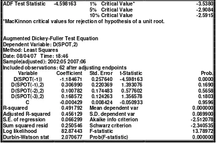
ADF Test Statistic -4.598163 1% Critical Value* -3.5380

5% Critical Value -2.9084

10% Critical Value -2.5915

*MacKinnon critical values for rejection of hypothesis of a unit root.

Augmented Dickey-Fuller Test Equation Dependent Variable: D(SPOT,2)

Method: Least Squares Date: 08/04/07 Time: 18:46

Sample(adjusted): 2002:05 2007:06

Variable Coefficient Std. Error t-Statistic Prob.

D(SPOT(-1)) -1.184671 0.257640 -4.598163 0.0000

D(SPOT(-1),2) 0.306990 0.220369 1.393076 0.1690

D(SPOT(-2),2) 0.100782 0.174483 0.577602 0.5658

D(SPOT(-3),2) 0.168572 0.124263 1.356578 0.1803

C -0.000429 0.008424 -0.050933 0.9596

[image:18.595.68.497.73.357.2]

Table 3 Augmented Dickey-Fuller Unit Root Test on D(SPOT)

Dependent Variable: DEPRECIATIONRATE Method: Least Squares

Date: 08/03/07 Time: 10:11

Sample(adjusted): 2002:01 2007:06

C -0.001091 0.010794 -0.101052 0.9198

IDIFF2 0.001508 0.460469 0.003275 0.9974

R-squared 0.000000 Mean dependent var -0.001061 Adjusted R-squared -0.015625 S.D. dependent var 0.045476 S.E. of regression 0.045830 Akaike info criterion -3.297915 Sum squared resid 0.134426 Schwarz criterion -3.231562

Log likelihood 110.8312 F-statistic 1.07E-05

[image:18.595.73.494.411.593.2]

(19)

3 0 2 4 6 8 10 12

-0.10 -0. 05 0.00 0.05 0.10 0.15

Series: Residuals Sample 2002:01 2007:06 Observations 66

Mean 1.52E-18 Median -0.008922 Maximum 0.151080 Minimum -0.098959 Std. Dev. 0.045476 Skewness 0.803639 Kurtosis 4.681580

[image:19.595.72.387.69.229.2]

Jarque-Bera 14.88041 Probability 0.000587

Table 5 UIP regression residuals histogram analysis

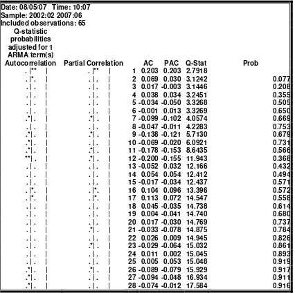
Date: 08/05/07 Time: 10:01 Sample: 2002:01 2007:06 Included observations: 66

Autocorrelation Partial Correlation AC PAC Q-Stat Prob

[image:19.595.72.495.282.667.2]

. |*******| . |*******| . |*******| . |****** | . |****** | . |****** | . |***** | . |***** | . |***** | . |**** | . |**** | . |**** | . |*** | . |*** | . |** | . |** | . |** | . |*. | . |*. | . | . | . | . | . | . | . | . | .*| . | .*| . | .*| . | .*| . | **| . | . |*******| 1 0.948 0.948 62.000 0.000 . | . | 2 0.896 -0.021 118.27 0.000 . | . | 3 0.845 -0.019 169.10 0.000 . | . | 4 0.801 0.046 215.57 0.000 . | . | 5 0.765 0.051 258.66 0.000 . | . | 6 0.729 -0.023 298.43 0.000 .*| . | 7 0.688 -0.064 334.43 0.000 . | . | 8 0.647 -0.011 366.85 0.000 . | . | 9 0.606 -0.024 395.78 0.000 . | . | 10 0.563 -0.053 421.18 0.000 . | . | 11 0.517 -0.056 443.02 0.000 . | . | 12 0.476 0.010 461.84 0.000 .*| . | 13 0.429 -0.084 477.41 0.000 .*| . | 14 0.376 -0.100 489.60 0.000 . | . | 15 0.323 -0.035 498.80 0.000 .*| . | 16 0.265 -0.100 505.09 0.000 . | . | 17 0.208 -0.048 509.04 0.000 . | . | 18 0.156 -0.009 511.32 0.000 . | . | 19 0.105 -0.037 512.37 0.000 . | . | 20 0.062 0.024 512.75 0.000 . | . | 21 0.021 -0.012 512.79 0.000 . |*. | 22 -0.010 0.078 512.80 0.000 . | . | 23 -0.043 -0.026 512.99 0.000 . | . | 24 -0.077 -0.045 513.62 0.000 . | . | 25 -0.113 -0.029 515.01 0.000 . | . | 26 -0.144 0.027 517.32 0.000 . | . | 27 -0.173 -0.025 520.75 0.000 . | . | 28 -0.196 0.015 525.29 0.000

(20)

4

Date: 08/05/07 Time: 10:07 Sample: 2002:02 2007:06 Included observations: 65

Q-statistic probabilities adjusted for 1 ARMA term(s)

Autocorrelation Partial Correlation AC PAC Q-Stat Prob . |** | . |** | 1 0.203 0.203 2.7918

[image:20.595.73.499.70.494.2] [image:20.595.70.496.551.739.2]

. |*. | . | . | 2 0.069 0.030 3.1242 0.077 . | . | . | . | 3 0.017 -0.003 3.1446 0.208 . | . | . | . | 4 0.038 0.034 3.2451 0.355 . | . | . | . | 5 -0.034 -0.050 3.3268 0.505 . | . | . | . | 6 -0.001 0.013 3.3269 0.650 .*| . | .*| . | 7 -0.099 -0.102 4.0574 0.669 . | . | . | . | 8 -0.047 -0.011 4.2283 0.753 .*| . | .*| . | 9 -0.138 -0.121 5.7130 0.679 .*| . | . | . | 10 -0.069 -0.020 6.0921 0.731 .*| . | .*| . | 11 -0.178 -0.153 8.6435 0.566 **| . | .*| . | 12 -0.200 -0.155 11.943 0.368 . | . | . | . | 13 -0.052 0.032 12.166 0.432 . | . | . | . | 14 0.054 0.054 12.412 0.494 . | . | . | . | 15 -0.017 -0.034 12.437 0.571 . |*. | . |*. | 16 0.104 0.096 13.396 0.572 . |*. | . |*. | 17 0.113 0.072 14.547 0.558 . | . | . | . | 18 0.045 -0.035 14.738 0.614 . | . | . | . | 19 0.004 -0.041 14.740 0.680 . | . | . | . | 20 0.017 -0.030 14.769 0.737 . | . | .*| . | 21 -0.033 -0.078 14.875 0.784 . | . | . | . | 22 0.026 0.009 14.945 0.826 . | . | .*| . | 23 -0.029 -0.064 15.032 0.861 . | . | . | . | 24 0.011 0.002 15.045 0.893 . | . | . | . | 25 0.005 0.053 15.048 0.919 .*| . | .*| . | 26 -0.089 -0.079 15.929 0.917 .*| . | . | . | 27 -0.094 -0.048 16.934 0.911 .*| . | . | . | 28 -0.074 -0.012 17.584 0.916

Table 7Correlogram of residuals obtained from the AR(1) model of UIP deviation

Dependent Variable: DEVIATION Method: Least Squares

Date: 08/05/07 Time: 18:33

Sample(adjusted): 2002:02 2007:06

Included observations: 65 after adjusting endpoints Convergence achieved after 4 iterations

C -0.622906 0.493088 -1.263275 0.2111

AR(1) 0.957440 0.011302 84.71612 0.0000

R-squared 0.991298 Mean dependent var -1.955385 Adjusted R-squared 0.991160 S.D. dependent var 1.191284 S.E. of regression 0.112006 Akaike info criterion -1.510243 Sum squared resid 0.790356 Schwarz criterion -1.443339

Durbin-Watson stat 1.594068 Prob(F-statistic) 0.000000 Inverted AR Roots .96

(21)

5

ARCH Test:

F-statistic 2.996140 Probability 0.037962

Obs*R-squared 8.319080 Probability 0.039858

Test Equation:

Dependent Variable: RESID^2 Method: Least Squares Date: 08/05/07 Time: 19:07

Sample(adjusted): 2002:05 2007:06

C 0.008157 0.003294 2.476317 0.0162

RESID^2(-1) 0.130386 0.125591 1.038181 0.3035

RESID^2(-2) 0.319694 0.120481 2.653477 0.0103

RESID^2(-3) -0.149345 0.125367 -1.191262 0.2384

[image:21.595.71.497.71.320.2]

Table 9ARCH Test of UIP deviation

Dependent Variable: DEVIATION Method: ML – ARCH

Date: 08/05/07 Time: 19:11

Sample(adjusted): 2002:02 2007:06

Included observations: 65 after adjusting endpoints Convergence achieved after 39 iterations

Coefficient Std. Error z-Statistic Prob.

C -0.384017 0.335510 -1.144576 0.2524

AR(1) 0.949655 0.007124 133.2955 0.0000

Variance Equation

C 0.001141 0.000853 1.337222 0.1812

ARCH(1) 0.531462 0.301554 1.762410 0.0780

GARCH(1) 0.468985 0.191401 2.450272 0.0143

R-squared 0.990859 Mean dependent var -1.955385 Adjusted R-squared 0.990249 S.D. dependent var 1.191284 S.E. of regression 0.117635 Akaike info criterion -1.568260 Sum squared resid 0.830283 Schwarz criterion -1.401000

Durbin-Watson stat 1.505745 Prob(F-statistic) 0.000000 Inverted AR Roots .95

[image:21.595.70.498.376.611.2]