Iterative Bilateral Filter and Non Local Mean

Iterative Bilateral Filter and Non-Local Mean

Dao Nam Anh

Department of Information Technology Electric Power University 235 Hoang Quoc Viet road

Hanoi, Vietnam

ABSTRACT

Using local or non-local features has proven to be a competent approach for denoising images. As noise and edges have similar effect of changes in gradient in many cases, noise allocation for denoising is still significant challenge. This work addresses the classic problem but introducing the combination concept of local and non-local factors with deviation refinement procedure. A new algorithm of the concept is proposed to ameliorate noise reduction. Sensitivity of noise detection is examined by iterative non-local mean and bilateral filter with refinement of range deviation. The final methodology is tested with Gaussian noise and compared with both non-local mean, bilateral filter. Experiment demonstrates improvement of denoising level in the new algorithm.

General Terms

Pattern Recognition, Algorithms.

Keywords

Image denoising, non-local mean, bilateral filter, noise deduction, iterative filter.

1.

INTRODUCTION

Image are corrupted by variable noise methods and denoising is essential task for image enhancement. Each pixel in the image must be examined if noise exists. This task is practical important because noise affects to object detection and scene understanding. Existing denoising methods have different strengths and weakness. Some filters remove noise but can not keep edges.

Noise and edges usually have the same effect of changes in gradient. In case when edges are seen like noise, edges are removed by the denoise operators and image becomes over-smooth. So detection of noise from edges is significant challenge for image enhancement.

Sigma-based operators like non-local mean and bilateral filer have been introduced for solving the problem. Initial versions of non local mean operators [1],[2],[3],[4] met numerous further research for improvement of denoising quality and performance. It was studied also for other image applications like demosaic [5], image compression [6], image inpainting [7]. Bilateral filter [8] have also been developed to many applications [9], [10].

This work have pursued an approach with some success to improve noise deduction but keep well edges. A new proposed algorithm was based on combination of non-local mean and bilateral filter for iterative noise detection. Intensive variation of bilateral filter is refined in each iteration by noise estimation which is determined by non-local and local factors. Experimental results present improvement of edges keeping for above sigma-based operators.

2.

OUTLINE OF PAPER

The remainder of this paper is organized as follows. Detailed literature review is presented in Sec. 3. A new proposed non-local approach is explained in detail in Sec. 4. Implementation of IBFNM algorithm for gray and color image is elaborated in Sec. 5. Discussion of the advantages and drawbacks of this approach is presented in Sec. 6. Future working is in Sec. 7 with pointers to Conclusion in Sec. 8.

3.

PRIOR WORK

Image features can be local, global and non-local (NL). The concept neighborhood filters introduced by Yaroslavsky [2]. Average is taken from neighbors having similar value to regarding pixel. Examplar-based inpainting use similar patches with the position of losing information to fill in [3]. This approach received numerous further development. Some works proposed methods for improvement of denoising output.

Kervrann et al [11] proposed a weighted sum of data points within an adaptive neighborhood for each pixel. The weighted sum balances the accuracy of approximation and the stochastic error.

The others link non-local mean with bilateral filter [9], [12]. A common weighted average filter [10] is introduced by Tanaka et al. It interprets bilateral filter and the NL-means filter like patch-based posterior mean with high-order Markov Random Fields (MRF) prior, that is learned by the locally adaptive prior learning. image patches by learned basis functions is presented like a denoising framework by Chatterjee et al [13].

A modified bilateral filtering is defined by Alonso-González et al [14] in terms of spatial and polarimetric distances. These distances encapsulate knowledge in both domains for an adaptation to the data structure. The method used an iterative weight refinement procedure, employing the filtered images to compute a more reliable estimation of the filter weights.

4.

ITERATIVE FILTER

4.1

Non-Local Filter

Removing noise from image is a classic signal processing problem. In additional noise model, noise image u is result of addition of noise n to original image v:

) ( ) ( )

(x v x n x

u   (1)

Image

v

needs to be recovered from input image

u

. Neighborhood filter proposed by Yaroslavsky [2] selects a set of pixels J(x) for each pixel x in input image . The set is defined by spatial close to x and similarity of intensive value with u(x). Mean of u for pixels of the set

) (x

J in discrete form is applied for all pixels:







)

( ( )

| ) ( |

1 ) (

x J y

u u y

x J x

NH (2)

Lindenbaum et al addressed the Gaussian filter _G which is a smoothing filter but at the cost of less distinct edges [15]:

      

 2₂

2 exp 2 1 ) (   

 x x

G (3)

The Gaussian filter then became a base for other filters, that are called by other way - sigma-filters. NL-means by Buades et al [16], [17] has a formula quite similar to the sigma-filter [8], [9]):





 w x yu ydy x

C x

NM_u ( , ) ( )

) ( 1 ) ( (4)

where similarity weight function w(x,y) depends on similarity of pixels

x

andy[16] using (3):

) ) .) ( .) ( ( exp( ) , ( ₂ 2 h y u x u G y x

w      

(5)

and C(x) is the normalization factor over neighbors N(x):



 ) ( ( , ) ) ( x

N w x ydy

x

C (6)

Non-local neighborhood filters for color images [2], [4] get similar intensive mean (2). Pixels with similar color B_p(x)

take their average in _L2_{exponent form:}



   ) ( 2 2 ) ( ) ) ( ) ( exp( ) ( 1 ) ( x B u p dy y u h x u y u x C x NF (7)

Only pixels in B_p(x) are averaged whereh manages the color similarity and _C(x) is the normalization factor.

4.2

Bilteral Filter

Bilateral filter (BF) is introduced by Tomasi and Manduchi [8], with frame size



, global space deviation



_s and range

deviation



_r which makes surfaces smooth, just as the Gaussian filter, while maintaining sharp edges better than the Gaussian filter (3):



x y



G



u x u y



u ydy G W u BF x N y x x r s



    ) ( || || ( ) ( ) ( ) 1 ] [    (8)

where

W

(

x

)

is the normalization factor:



x y



G



u x u y



dy G

x W

x N

y s r



    ) ( || || ( ) ( ) ) (    (9)

Bilateral filter takes pixels in a frame (size



) around the pixel and uses local intensive information of the frame to perform (8).

4.3

Noise and Edges

Noise and edges have common sign of high gradients uin L norm:             

x u, u ,x (10)

image details are loss in results. The gray levels are flatten after each level of wavelet reconstruction, resulting in a cartoon-like appearance.

4.4

NOISE DETECTION BY TWO

VIEWS

Addressing the losing some image details in BF filter this section proposes a new approach for noise detection by both NM-mean and BF filter. Our main idea is to detect noise under different points of view. Noise assumptions are different under NM-mean and BF filter, thereby confidence of noise detection must be better when use the both methods, thought it takes additional computational cost.

Firstly, from the view of NL-mean, difference of u(x)and output of filter _NMu(x) supports to get probability on location of noise by the filter:

) /( ) ( )

(n  NM u u u



PNM (11)

where



0is to prevent division by zero.

Secondly, similarly for BF, probability on noise location by bilateral filter has following form:

) /( ) ( )

(n  BF u u u



PBF ₍₁₂₎

Average of above probabilities gives better noise assumption than self NL mean or self BF:

)) ( ) ( ( ) ( 2

1 _{P n P n}

n

PNMBF  NM  BF ₍₁₃₎

) /( * 2 ) ( ) ( )

(_n ₂1 _{NM u} _{BF u}  _{u u}



PNMBF 1 ) /( )) ( ) ( ( ) ( 2

1   

 NM u BF u u



n

PNMBF ₍₁₄₎

This solution is simple but effective in practices, see examples in Fig. 2b, 2c, and 2d.

4.5

REFINEMENT FOR BF RANGE

DEVIATION

Original bilateral filter (8) applies predefined constant range deviation



_rthat could lead to blur the image thereby removing much of the image details. Our new solution for this problem is using found probability of noise to refine the BF range deviation. Iterative deviation refinement procedure will be applied to the solution, similar to the weight refinement procedure in [14]. Using probability of noise to update deviation can lead to better covering noise and keeping edges.

Initial range deviation



_r in (8) is a constant. However, the

adaptive version of sigma



_r

(

x

)

can be presented by a function dependent on noise probability for matching the noise assumption: ) ) )( ( /( ) (





x k PNMBF n x 

r (15)

Now the new denoising approach is an iterative procedure of filters for refinement of the BF range deviation.

] ; [ ) (

1   



r r t

r x







(17)





 _

x t r (x) 1

1



(18)

Condition (17) is to keep deviation average the same as it was given initially. Formula (18) is for Gaussian normalization.

Combining the solution from 4.4, denoised output image for each iteration is average of the two filters’ outputs: NM mean for non-local factors and BF for local factors. In the initial iteration,

))

(

)

(

(

0 2 1 0

u

BF

u

NM

v





(19)

In next iterations, the BF range deviation 1( )

x

t r





is refined by (16) and then

BF

t1

(

u

)

is calculated with the deviation

) ( 1 x t r 



. Output of the iteration is an average:

))

(

)

(

(

1 2 1 1

u

BF

u

NM

v

t





t (20)

Stop condition of the iterative procedure is based on variance function



t1_:

2

,

1

,

1

1









 

L

v

v

t t L

t ₍₂₁₎

The procedure is stopped when

t t







1 ₍₂₂₎

So, the described denoising approach is based on probabilities of noise delivered by NL mean and BF filters. This also applies refinement for BF range deviation by the noise assumption. The approach is resumed in the following section.

4.6

ALGORITHM IBFNM

The algorithm IBFNM is short for “Iterative Bilateral Filter and Non-local Mean”. It contains the following steps.

Start: given image , size



and initial standard deviation: 

  

const const x

x s

r( ) , ,

0





(23)

Calculate NM(u),BF0(u)with 0

r



, and then

v

0:

)) ( ) ( ( 0 2 1

0 _{NM u BF u}

v   (24)

At (t+1) iteration:

Find probability of noise location:

1 ) /( )) ( ) ( ( ) ( 2

1   

 NM u BF u u



n

Pt t ₍₂₅₎

Refine the BF range deviation:

) ) )( ( /( ) ( 1





   x n P k x t t r (26)

Calculate 1( ) u

BFt _with 1_{( )}

x

t r





and then

v

t1:

)) ( ) ( ( 1 2 1

1 _{NM u BF u}

vt   t ₍₂₇₎

Stop: when

t t







1

(28)

2

,

1

,

, 1

1

_

_

_



 

L

v

v

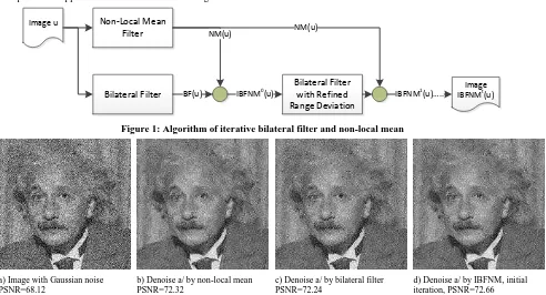
t t L

t ₍₂₉₎ Non-Local Mean Filter Bilateral Filter Bilateral Filter with Refined Range Deviation NM(u)

IBFNM0(u)

NM(u) Image u

BF(u)

Image IBFNMt_(u)

[image:3.595.61.553.397.663.2]

IBFNM1(u)…..

Figure 1: Algorithm of iterative bilateral filter and non-local mean

a) Image with Gaussian noise PSNR=68.12

b) Denoise a/ by non-local mean PSNR=72.32

c) Denoise a/ by bilateral filter PSNR=72.24

d) Denoise a/ by IBFNM, initial iteration, PSNR=72.66

e) Denoise a/ by IBFNM, 1rst iteration, PSNR=74.09

d) Denoise a/ by IBFNM, 2nd iteration, PSNR=74.27

d) Denoise a/ by IBFNM, 3rd iteration, PSNR=73.93

e) PSNR of results for a) by 3 iterations

Figure 2: Example of IBFNM for gray image.

a)Image with Gaussian noise PSNR=68.27

b)Denoise a/ by non-local mean PSNR=70.66

c) Denoise a/ by bilateral filter PSNR=70.18

d) Denoise a/ by IBFNM, PSNR=71.07, 2 iterations.

a)Gaussian noise PSNR=68.44 e)Denoise a/ by non-local mean PSNR=70.47

f) Denoise a/ by bilateral filter PSNR=70.18

g) Denoise a/ by IBFNM, PSNR=71.07, 2 iterations.

a)Gaussian noise PSNR=68.39 b)Denoise a/ by non-local mean PSNR=73.19

c) Denoise a/ by bilateral filter PSNR=71.15

a)Gaussian noise PSNR=68.90 b)Denoise a/ by non-local mean PSNR=70.79

c) Denoise a/ by bilateral filter PSNR=70.34

[image:5.595.58.548.73.225.2]

d) Denoise a/ by IBFNM, PSNR=71.13, 4 iterations.

Figure 3: Example of IBFNM for color images.

Figure 1 presents principal steps of the algorithm.

5.

EXPERIMENTS

PSNR is chosen to validate the superiority of the proposed algorithm IBFNL. Its performance is compared with NL-mean and BF by visual quality and PSNR.

5.1

GRAY IMAGE

An example of gray image run by the algorithm is demonstrated in Fig.2. Input image Fig.2a is corrupted by Gaussian noise with PSNR=68.12.

Results of NL-mean and BF are shown in Fig.2b, 2c with PSNR=72.32 and PSNR=72.24 accordingly.

There were 4 iterations for the input gray image with PSRNs: 72.66; 74.09, 74.27; 73.93, and it’s stopped after the 3rd iteration. Graph of PSNR for each iteration is in Fig.2e, showed that IBFNL gave the best result comparing with NM and BF, thought its 2nd step has given the best PSNR.

5.2

COLOR IMAGES

Color images from Segmentation Dataset and Benchmark of Berkeley Computer Vision group Berkeley were used to test the IBFNM algorithm. Results are demonstrated in Fig.3. Gaussian noise was added to the color images (Fig.3a). Results of NM-mean, BF and IBFNM are set on column Fig.3b, 3c and 3d. PSNR index is calculated for each cases. The superiority of IBFNM is validated from the examples.

6.

DISCUSSION

The algorithm IBFNM needs three initial parameters:



_s,



_r and BF’s frame size



. Parameters



_s,



_r regulate local Gaussian distribution of similarity weight. The frame size is to define local space that is used to estimate noise location in step 2 of the algorithm (formula 23, and 24). Too small or too big frame size could lead to over-noise or over-edges.

Similar solution to the range deviation



_r(x) is making the space deviation



_s(x)and frame size



(x) adaptive to probability of noise:

) ) )( ( /( ) (

1





  

x n P k

x s t

t

s (30)

) ) )( ( /( ) (

1





t _x _{k P}t _{n x}  ₍₃₁₎

In addition, calculation of 1_{( )}

x

t s





and



t1(_x) _{by (30) and}

(31) will be new tasks of the IBFNM algorithm, their position is next after formula (26). The algorithm gives results that keeping edges, thought it needs more time for iterations of non-local mean and BF filter.

7.

FUTURE WORK

Noise models and types of original images could lead to variable mix of noise and edges. Intention to detect noise from edges is needed to check carefully noise models and image types. Parameters of above algorithms depend on nature of the noise and input image. Study for these questions could be a way for further development of the iterative algorithms.

8.

CONCLUSION

An adaptive version of BF and non local mean for de-noising is presented in the paper. In this version, probability of noise is addressed in order to keeps edges well during denoising by non local and local operators. The new iterative IBFNM algorithm makes BF standard deviation adaptive to the probability of noise. Experimental results shows remarkable improvement of noise reduction of the new algorithms. Gaussian noise model are reduced by the algorithm.

9.

ACKNOWLEDGMENTS

Author thank Berkeley Computer Vision group for the Berkeley Segmentation Dataset and Benchmark, its images were used in fig. 1 and fig. 2 in this article. Special thank Gabriel Peyré for his toolbox of nlmeans [19] with which codes for this article started. Author would also like to thank the internal reviewers at EPU and the anonymous referees for their valuable comments.

10.

REFERENCES

[1] P. Arias, V. Caselles, G. Facciolo, Analysis of a Variational Framework for Exemplar-Based Image Inpainting.

[2] L.P. Yaroslavsky, Digital Picture Processing - An Introduction, Springer Verlag, 1985.

[3] A.A. Efros and T.K. Leung. Texture synthesis by non-parametric sampling. In Proc. of the IEEE Conf. on CVPR, pages 1033–1038, Corfu, Greece, 1999.

[4] J.S. Lee, Digital image smoothing and the sigma filter, Computer Vision, Graphics and Image Processing, vol. 24, pp. 255-269, 1983.

[5] Pablo Arias, Vicent Caselles, and Guillermo Sapiro, A Variational Framework for Non-local Image Inpainting.

[6] Steffen Börm, Efficient Numerical Methods for Non-local Operators: H2-Matrix Compression, Algorithms and Analysis, EMS Tracts in Mathematics, 2010; 441 pp.

[8] C. Tomasi and R. Manduchi. Bilateral filtering for gray and color images. In Proc. of the Sixth International Conference on Computer Vision, Bombay, India, 1998.

[9] Sylvain Paris and Fredo Durand, A Fast Approximation of the Bilateral Filter using a Signal Processing Approach, CSAIL, MIT, 2006.

[10]S. Paris, P. Kornprobst, J. Tumblin and F. Durand, Bilateral Filtering: Theory and Applications in Computer Graphics and Vision Vol 4, No.1 (2008).

[11]C. Kervrann and J. Boulanger, Optimal Spatial Adaptation for Patch-based Image Denoising, IEEE Trans. on Image Processing 15(10) 2866-2878 (2006).

[12]L. Rudin, S. Osher, and E. Fatemi, Nonlinear total variation based noise removal algorithms, Phys. D, 1992.

[13]Kwok-Wai Hung and Wan-Chi Siu, Real time interpolation using Bilateral filter for Image zoom or Video up-scaling/transcoding, ICCE 2012, pp. 67-68.

[14]A Alonso-González, C López-Martínez, P Salembier, X Deng, Bilateral Distance Based Filtering for Polarimetric SAR Data, Remote Sensing 5 (11), 5620-5641, 2013

[15]M. Lindenbaum, M. Fischer, and A. M. Bruckstein, On Gabor’s contribution to image enhancement, Pattern Recognition, 27 (1994), pp. 1–8.

[16]A. Buades, B. Coll and J.M. Morel, A non-local algorithm for image denoising, IEEE Int. Conf. on Computer Vision and Pattern Recognition, 2005.

[17]A. Buades, B. Coll, J.M Morel, Nonlocal Image and Movie Denoising, International Journal of Computer Vision, Vol 76 (2), pp: 123-139, 2008.

[18]M. Zhang, B.K. Gunturk, Multiresolution Bilateral Filtering for Image Denoising, IEEE Trans. Image Process. Vol.17 (2008), p. 2324.