Munich Personal RePEc Archive
Implications of Oil Price Shocks for
Monetary Policy in Ghana: A Vector
Error Correction Model
Tweneboah, George and Adam, Anokye M.
School of Management, University of Leicester
2008
Implications of Oil Price Shocks for Monetary Policy in Ghana: A
Vector Error Correction Model
George Tweneboah
School of Management, University of Leicester, UK. E-mail: gt56@le.ac.uk
Anokye M. Adam
School of Management, University of Leicester, UK. E-mail: ma262@le.ac.uk
Abstract
We estimate a Vector Error Correction Model to explore the long run and short run linkages
between the world crude oil price and economic activity in Ghana for the period 1970:1 to
2006:4. The results point out that there is a long run relationship between the variables under
consideration. We find that an unexpected oil price increase is followed by an increase in price
level and a decline in output in Ghana.We argue that monetary policy has in the past been with
the intention of lessening negative growth consequences of oil price shocks, at the cost of higher
inflation.
Key words: Oil price shock, cointegration, vector error correction, impulse response
1.Introduction
The world crude oil market has witnessed profound fluctuations over the past few decades,
rocketing to a record $147 per barrel in July 2008. This persistent oil price shocks could have
severe macroeconomic implications and present crucial challenges for policymaking, and makes
it essential to empirically understand their effects on economic activity in especially
oil-importing developing countries such as Ghana.
The effect of oil prices on economic activity has received a plethora of theoretical and empirical
research in the past few decades. According to an influential contribution by Hamilton (1983), all
but one of U.S. economic downturns since World War II had been preceded by oil price hikes,
indicating an inverse relationship between oil price shocks and aggregate economic activity as
documented in most earlier studies on the U.S. economy (see, inter alia, Rasche and Tatom,
1977; Mork and Hall, 1980). Other studies report similar inverse relationships for other countries
(See, for example, Papapetrou (2001) for Greece, Cunado and Perez de Gracia (2003) for EU and
de Miguel, Manzano, and Martin-Moreno (2003) for Spain.
It was assumed that since oil price increases slow down economic activity, falling oil prices
should stimulate macroeconomic performance until it was established by some studies that
economic activity reacts asymmetrically to oil price shocks (see, Mork, 1989; Ferderer, 1996).
Others have attributed this to the contractionary monetary policy pursued by most central banks
in response to oil price hikes (Bernanke, Gertler and Watson, 1997).
The literature has made several attempts to explore the mechanisms through which oil price
input to production, an increase in oil price give rise to increased production costs which causes
productivity to decline. Oil price hikes reduces the spending power of consumers and encourage
producers to substitute less energy intensive capital for more energy intensive capital. The
literature predicts that the magnitude of this effect depends on whether the shock is transitory or
permanent in nature.Consequently, the different authors have assigned weights to the supply and
demand channels (see, for example, Rasche and Tatom, 1977, 1981; Kim and Loungani, 1992;
Rotemberg and Woodford, 1996; Abel and Bernanke, 2001). Other channels include the real
balance effect (see Pierce and Enzler, 1974; Mork, 1994), and the transfer of income from oil
importing countries to oil exporting countries through deteriorating terms of trade (Dohner,
1981).This transfer of wealth leads to a decrease in global demand in the oil-importing countries
which outweighs the increase in the oil-exporting countries because of the assumed low
propensity to consume in the latter.
The objective of this paper is to explore the effects of oil price shocks on macroeconomic
variables such as output and prices in Ghana and how monetary policy has in the past contributed
to the impact of this shock. The rest of the paper is set out as follows. Section 2 gives a brief
overview of the role of oil prices and the recent performance of the Ghanaian economy. Section
3 presents the methodology while Section 4 discusses the empirical results. Section 5 is the
summary and conclusion.
2. Oil Prices and Recent Economic Performance in Ghana
Researchers have argued that oil prices chiefly affect the macroeconomy as an import price,
costs or by increasing uncertainty which lead to deferral of irreversible investment; as a shock to
the aggregate price level which reduces real money stock, and as a relative price shock which
leads to costly reallocation of resources across sectors. These are further influenced by such
country specific factors as price controls, taxes on petroleum products, exchange rate fluctuations
and variations in domestic price index. From this one can argue that understanding the
relationship between the world oil price and economic activity is important because oil price
increases lead to a rise in prices of petroleum products which serve as a key production inputs
and as an essential consumer goods. These price increases are considerable enough that they
normally become temporary rise in the general rate of inflation. To the extent that increases in
the oil price lead to a rise in price level, purchasing power is also reduced through a reduction in
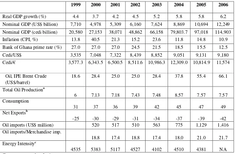
the real money stock. The energy intensity which measures the total primary energy consumption
per dollar of gross domestic product (using purchasing power parities) stayed at 4381 in 2005.
The economy of Ghana has grown at an average annual rate of about 4.7% over 1990-2007. This
growth rate has assumed an upward trend averaging around 6% from 2003-2007 following a
growth rate of 3.7% in 2000. This improving macroeconomic performance hastranslated into an
average annual per capita GDP growth of around 2.6% over 2000-2005 compared to 1.8% for
sub-Saharan Africa over the same period. The growth expansion has been driven principally by
significant boost in the agriculture sector, leading to an increased contribution to GDP of nearly
38% in 2006, supported by productivity increases and favourable international market cocoa
Inflation in Ghana has also decreased over the years from a high of around 71% in 1995 it has to
as low as around 10.9% at the end of 2006. Particularly, this decrease in inflation has been
achieved in the last six years due to tighter monetary policy following the increasing
independence of the Bank of Ghana. The exchange rate seems to be relatively stabilised
considerably against the major trading currencies over the years, translating into a substantial
reduction in annual depreciation rates much lower than inflation rates. This has raised some
concerns regarding the effects of the real appreciation of the exchange rate on the real economy
(particularly the manufacturing sector).
The implications of an oil price shock on an economy depend to a large extent on the importance
of oil as factor of production (LeBlanc and Chinn, 2004) and the state of the macroeconomy.
Crude oil is a very important factor of production which has led the government to subsidize
petroleum product prices to an estimated annual average of 2.3 percent of GDP until 2005. This
is reflected in the table as the consumption of oil has increased from about 27 thousand bbl
per/day in 1995 to 47 thousand bbl/day in 2005. Out of this about 39 thousand bbl were imported
per day which accounted for up to over 21% of total imports for the fiscal year, implying that
unexpected increases in world oil prices can adversely affect the terms of trade and the real
economy.
3. Data and Methodology
3.1. Data Description
Most studies that examine the oil price-macroeconomy relationship include a measure of
monetary policy stance. We follow that practice and analyse quarterly data for Gross Domestic
Product (GDP), Consumer Price Index (CPI), Interest rate (INT), bilateral U.S. dollar per Ghana
cedi Exchange Rate (NER) and World Crude Oil Prices (POIL) covering the period
1970:1-2006:4. With the exception of the Gross Domestic Product, all the data were quarterly and
obtained from the International Monetary Fund’s International Financial Statistics (IMF IFS)
July 2008 edition. Annual GDP data (at constant 2000 USD prices) was obtained from the April
2008 World Development Indicators (WDI) published by the World Bank and interpolated by
the technique suggested by Lisman and Sandee (1964). Opinions diverge on the best
specification of oil price including different and advanced stances such as “oil prices by
themselves do not have significant macroeconomic effects” (Bohi 1991), “oil price increases
matter but decreases do not” (Mork 1989), “oil price increases matter if they are large enough
relative to past experience” (Hamilton 1996), and “the effects oil price increases are a function of
their size relative to their current degree of variability” (Lee, Ni and Ratti 1995).This has led to
different measures of oil price shocks in the literature including the logarithm of oil price series
in levels, the first differences of oil prices, the positive oil price changes and the Net Oil Price
Increase (NOPI) proposed by Hamilton (ibid). The NOPI takes into account oil price changes
only if the percentage increase in price is above the observed values for the previous four periods
and zero otherwise. This measure eliminates price increases that simply correct price volatility to
capture more effectively the surprise element, which may be at the origin of a change in
spending decisions by firms and households. In this study, we include the logarithm of the
average U.S. dollar price of world crude oil to capture the linear oil-output relationship.
Analysis of the long-run relationship between non-stationary variables has become very critical
in multivariate time series literature. As revealed by Engle and Granger (1987), if the linear
combination of two or more non-stationary variables is stationary, then there is a long-run
relationship among the variables. The presence of cointegrating vector forms the basis of the
vector error correction model. In this study we utilize the Johansen (1991, 1995) methodology to
estimate the long-run cointegrating relation from a vector error correction model of the form:
(1)
∑
− = − − + + Π + Δ Γ = Δ 1 1 k j t k t j t j
t Z Z
Z μ ε
where Ztis a vector of endogenous I (1) variables/a (p×1) vector of variables integrated of
order 1, Δis the first difference lag operator, Γjis a (p×p) matrix that represents short-term
adjustments among variables across p equations at the j th lag, Π=−(I−A1−...−Ak), I is an
identity matrix whose rank determines the number of distinct cointegrating vectors. It could be
decomposed into the (n×r) matrix αand βsuch thatΠ=αβ'. αis a (p×r) matrix of the
speed of adjustment parameters to/speed of error correction mechanism, β'is (p×r) matrix of
cointegrating estimates of the long-run cointegrating relationship between the variables in the
model, μis a (p×1) vector of constants, and εtis a(p×1) vector of white noise error terms.
Johansen (1988) and Johansen and Juselius (1990) derived the likelihood ratio test for the
hypothesis thatΠ=αβ'. The cointegrating rank, r, can be formally tested with the trace test and
maximum eigenvalue test statistics proposed by the Johansen methodology. The short run
mechanics of the error correction model can be analysed through the impulse response and the
error correction term (ECT). The ECT determines the speed of adjustment due to each of the
4. Empirical Results
4.1 Stationarity and Long-Run Relationships
The objective of this paper is to explore the effects of oil price shocks on macroeconomic
variables such as output and prices in Ghana and how monetary policy has in the past contributed
to the impact of this shock. Since the cointegration methodology assumes that the variables be
integrated of the same order, we begin the empirical analysis with unit root tests in order to
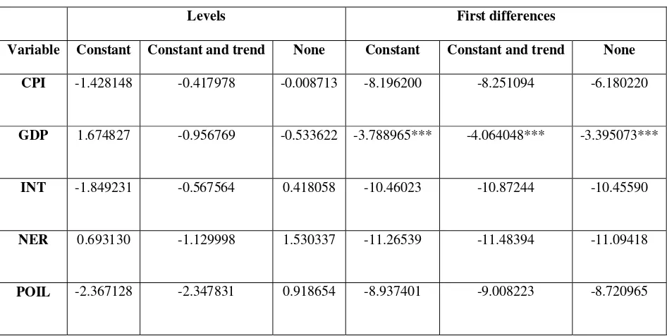
identify the stochastic trends of the series. We employ the Augmented Dickey-Fuller and
Phillips-Perron tests which are two of the most widely applied unit root tests. The results as
shown in Table 2 indicate that all the variables are integrated of order one, [I (1)]. This means
that we can utilize the cointegration technique to investigate whether there is a common
stochastic trend between the variables. The existence of cointegration would imply a long-run
equilibrium relationship between the variables under consideration. On the other hand, if we find
no cointegration we can specify a VAR in levels to investigate the short-run dynamics of the
variables.
As a key requirement in cointegration test, we proceed with the selection of the optimal lag
length for the specification of the model. In this study we accept the SIC as a guide to select the
lag length. The selection of this common lag length comes with it the misspecification hitch as
there are some trade-offs associated with the various information criterion employed in its
selection. This includes the choice between strongly consistent criteria such as the SIC and the
HQC on the one hand, and the less parsimonious AIC. The SIC is inclined to underestimation,
while there is increased cost for loss of degrees of freedom on the addition of more lags.In this
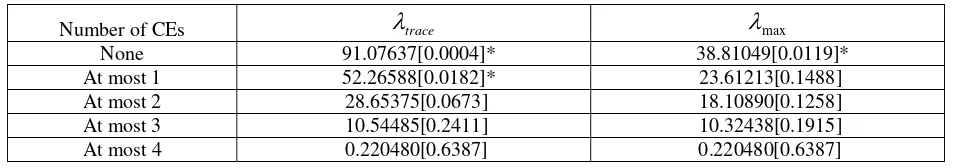
Following the lag order selection, we proceed to the cointegration analysis which is performed
by specifying an intercept with no trendfor the cointegrating equations. The cointegration test as
reported in the Table 3a reveals that all the variables under consideration; prices, GDP, interest
rates, exchange rate and world crude oil prices, share a common stochastic trend. This implies
that the following Vector Error Correction Model (VECM) can be estimated to capture the long
run as well as the short run dynamics:
(2) Δyt =Πyt−1+Γ1Δyt−1+...Γp−1Δyt−p+1+ut
This is obtained by subtracting yt−1from both sides of a reduced form standard VAR (p) model:
(3) yt =A1yt−1+...+Apyt−p +ut
where yt is a k×1vector of time series and A1,...,Apare k×kcoefficient matrices. The
reduced form disturbance ut is an k×1unobservable white noise process.
Table 3 indicates that there exists a long-run equilibrium relationship among the variables. In
both cases, all the coefficients are statistically significant. Interest rate and crude oil prices are
negatively correlated with GDP in the long run as shown in the following equation (standard
errors are in parentheses):
(4) (0.07) (0.05) (0.08) (0.07) 4 . 0 1 . 0 int 5 . 0 3 .
0 t t t t
t cpi ner poil
gdp = − + −
With this relationship, we can interpret that, in the long run a one percent increase in oil price
With inflation as the dependent variable, we find that all the variables are positively correlated
with inflation except exchange rates which is negatively correlated in the long run relationship
shown below (with standard errors in parentheses):
(5) (0.13) (0.11) (0.29) (0.83) 2 . 1 3 . 0 int 6 . 1 9 .
2 t t t t
t gdp ner poil
cpi = + − +
With this one can say that, in the long run, a percentage increase in oil price causes the price
level to rise by 1.2%.
4.2 Impulse Response Functions and Speed of Adjustment
In this section we follow the impulse response function to examine the short-run dynamics of the
model. This can be achieved by investigating the dynamic effects of a generalised one standard
deviation innovation on oil price, and the effects of a contractionary monetary policy response on
the other variables. In this case we expect a central bank mandated to stabilize prices to increase
interest rates in response to oil price hikes at the expense of output growth. The generalized
impulse response function employed in this study does not take into consideration the order of
the variables is the VECM and covers up to 24 quarters.
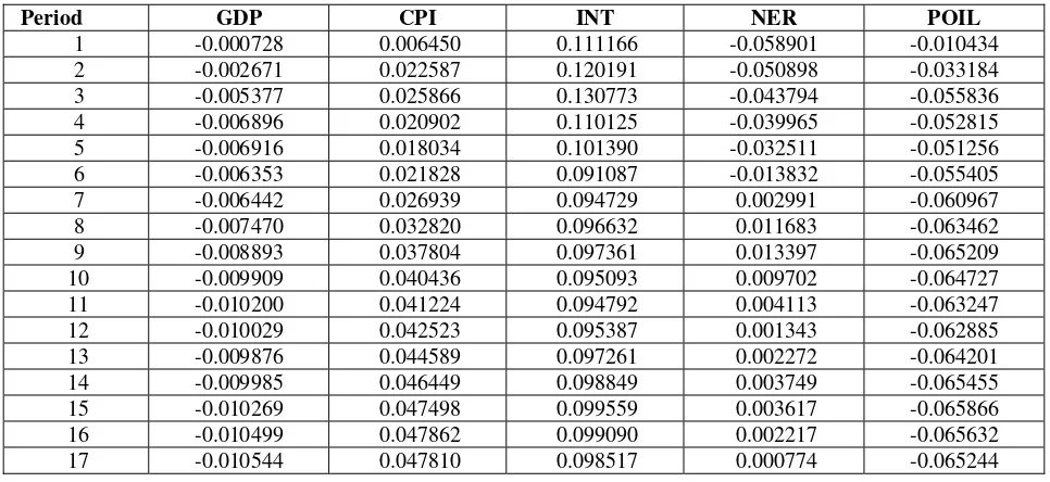
The impulse response functions displayed in Table 4 indicate that a generalised one standard
deviation shock to oil price causes prices to rise instantly to about 0.001% within two years.
Although prices react instantly and persists over a long horizon, output does not fall until after 4
quarters, which continues for a very long time hovering around 0.02% below its baseline. On the
response of monetary policy, the figure indicates that interest rates decline initially indicating
curtail further inflationary consequences of the oil price shock. The accumulated response (not
reported) shows that output falls by 0.36% while prices rise by almost 1% in 6 years. We argue
that the response of monetary authorities is not enough to mitigate the inflationary pressure
caused by the oil price shocks.
On the response of prices to a generalised one standard deviation shock to interest rates we can
say that contrary to our expectations, while output falls instantly prices rise. Prices rise from
0.006% in the first quarter to just about 0.05% within 6 years. The fall in output increases to
0.01% in 6 years. The accumulated response displays a 0.20% fall in output. Interestingly,
exchange rate appreciation does not lead to a fall in prices.
Since the impulse response function traces the effect of a one-time residual shock to an
innovation on current and future values of the endogenous variables, we consider the speed of
adjustment of the variablestowards the equilibrium relationship as part of the short run analysis.
From the table, we find that the adjustments due to GDP and nominal exchange rates play
significant roles in restoring the cointegrating relationship.
5. Summary and Conclusion
In this study we have estimated a vector error correction model to explore the long run and short
run linkages between the world crude oil price and economic activity in Ghana for the period
1970:1 to 2006:4. The results indicate that there is a long run relationship involving oil prices,
prices, GDP, exchange rate and interest rate in Ghana in which oil price positively impact the
price level while negatively impacting output. In the short run, we find that an unexpected oil
price shock is followed by an increase in inflation rate and a decline in output in Ghana. On the
past been with the intention of lessening any growth consequences of oil price shocks, but at the
cost of higher inflation.
The fact that oil price shocks impact the Ghanaian economy and the recent decision of the
government to eliminate subsidies on petroleum products and bring domestic petroleum prices
closer to world prices has important implications for monetary policy. For an effective inflation
targeting in Ghana, the credibility of monetary and fiscal policies should be improved and
properly coordinated so as to anchor inflationary expectations and mitigate any external shocks
on the economy.
References
Abel, A.B. and Ben S.Bernanke. 2001. Macroeconomics. Addison Wesley.
Bank of Ghana. Annual Report (various issues). Accra-Ghana.
Bernanke B.S., M. Gertler, and M. Watson. 1997. “Systematic Monetary Policy and the
Effects of Oil Price Shocks,” Brookings Papers on Economic Activity, 1, 91-142.
Bohi, D.R. 1991. “On the Macroeconomic Effects of Energy Price Shocks,” Resources and
Energy, 13, 145-62.
Cuñado, J. and Gracia, P. 2003. “Do oil price shocks matter? Evidence for some European
countries,” Energy Economics, 25 (2), 137-154.
De Miguel, C., B. Manzano and J.M. Martin-Moreno. 2003. “Oil Price Shocks and Aggregate
Dohner, R.S. 1981. “Energy prices, economic activity and inflation: survey of issues and
results,” in K. Mork (ed.) Energy Prices, Inflation and Economic Activity. Cambridge, MA:
Ballinger.
Engle, R.F. and C.W.J. Granger. 1987. “Co-integration and error-correction: Representation,
estimation and testing,” Econometrica, 55, 251-276.
Ferderer J.P. 1996. “Oil Price Volatility and the Macroeconomy,” Journal of Macroeconomics,
18, 1-16.
Hamilton, J. 1983. “Oil and the Macroeconomy since World War II,” Journal of Political
Economy, 91, 228-248.
Hamilton, J.D. 1996. “This is What Happened to the Oil Price-Macroeconomy Relationship,”
Journal of Monetary Economics, 38, 215-220.
International Monetary Fund. 2008. International Financial Statistics (IFS) April 2008. ESDS
International, University of Manchester.
Johansen, S. 1988. “Statistical analysis of cointegrating vectors,” Journal of Economic
Dynamics and Control, 12, 231-254.
Johansen, S. 1991. “Statistical Analysis of Cointegrating Vector,” in: Engle R. F., and Granger
C. W. J. (eds), Long-Run Economic Relationships. Oxford: Oxford University Press.
Johansen, S. 1995. “A Statistical Analysis of Cointegration for I (2) Variables,” Econometric
Theory, 11, 25–59.
Johansen S. and K. Juselius. 1990. “Maximum Likelihood and Inference on Cointegration with
Applications to the Demand for Money.” Oxford Bulletin of Economics and Statistics, 52,
Kim, I. and P. Loungani. 1992. “The Role of Energy in Real Business Cycle Models.” Journal
of Monetary Economics, 29, 173-189.
LeBlanc M. and M.D. Chinn. 2004. "Do High Oil Prices Presage Inflation? The Evidence from
G-5 Countries," UC Santa Cruz Economics Working Paper No. 561, SCCIE WP 04-04.
Lee, K., S. Ni, and R. Ratti. 1995. “Oil Shocks and the Macroeconomy: The Role of Price
Variability,” TheEnergy Journal, 18, 39-56.
Lisman, J.H.C. and J. Sandee. 1964. “Derivation of quarterly figures from annual data,”
Applied Statistics, 13, 87–90.
Mackinnon J.G., A.A. Haug and L. Michelis. 1999. “Numerical Distribution Functions of
Likelihood Ratio Tests for Cointegration,” Journal of Applied Econometrics, 14, 563-577.
Mork K.A. 1989. “Oil Shocks and the Macroeconomy when Prices Go Up and Down: an
Extension of Hamilton’s Results,” Journal of Political Economy, 97 (51), 740-744.
Mork, K.A. 1994. "Business Cycles and the Oil Market," Energy Journal, 15, 15-38.
Mork, K.A. and R.E. Hall. 1980. “Energy Prices, Inflation, and Recession, 1974-75.” The
Energy Journal, 1(3): 31-63.
Papapetrou, E. 2001. “Oil price shocks, stock market, economic activity and employment in
Greece,” Energy Economics, 23 (5), 511-532.
Pierce, J.L. and J.J. Enzler. 1974. “The Effects of External Inflationary Shocks,” Brookings
Papers on Economic Activity, 1, 13-61.
Rasche, H. R. and J. A. Tatom. 1977. "Energy resources and potential GNP," Review of
Federal Reserve Bank of St. Louis, June, 10-24.
Rotemberg, J.J., M. Woodford. 1996. “Imperfect Competition and the Effects of Energy Price
World Bank. 2008. World Development Indicators (WDI) April 2008. ESDS International,
Appendix
Table 1: Selected Economic Indicators
1999 2000 2001 2002 2003 2004 2005 2006
Real GDP growth (%) 4.4 3.7 4.2 4.5 5.2 5.8 5.8 6.2
Nominal GDP (US$ billion) 7,710 4,978 5,309 6,160 7,624 8,869 10,694 12,249 Nominal GDP (cedi billion) 20,580 27,153 38,071 48,862 66,158 79,803.7 97,018 114,903
Inflation (CPI, %) 13.8 40.5 21.3 15.2 23.6 11.8 14.8 10.9
Bank of Ghana prime rate (%) 27.0 27.0 27.0 24.5 21.5 18.5 15.5 12.5 Cedi/US$ 3,535 7,048 7,322 8,439 8,852 9,051 9,131 9,180
Cedi/€ 3,577.3 6,343.5 6,500.5 8,511.6 10,986.3 12,309.0 10,814.9 11,574
Oil, IPE Brent Crude (US$/barrel)
18.6 28.4 25.0 25.0 28.4 37.8 55.4 66.1
Total Oil Productiona
6 7.13 7.18 7.43 7.48 8.57 7.57 7.57 Consumption
31 37 36 39 42 45 47 49 Net Exportsb
-25 -30 -29 -31 -34 -37 -39 -42 Oil imports (US$ million) 520 517 510 563 775 1,129 1,416 Oil imports/Merchandise imp.
18.8 17.4 18.8 17.4 18.0 21.0 21.7 Energy Intensityc
4535 5383 5117 4527 4102 4510 4381 NA
Sources: Bank of Ghana
a Production of crude oil including lease condensate, natural gas plant liquids, and other liquids,
and refinery processing gain/loss. (Negative value indicates refinery processing loss)
b Total Oil Production minus Consumption (Negative numbers are Net Imports) c
Table 2: Unit Root Tests
a. Augmented Dickey Fuller Test
Levels First differences
Variable Constant Constant and trend None Constant Constant and trend None
CPI -1.762184 -0.164293 -0.387853 -5.242049 -8.241501 -2.312094**
GDP 1.051035 -2.210721 -0.315810 -4.303010*** -5.148314*** -3.368369***
INT -1.869860 -0.929947 0.331326 -10.51102 -10.65552 -10.51122
NER 0.733880 -1.107014 1.589207 -11.26765 -11.48394 -11.05938
POIL -2.569060 -2.648436 0.691604 -8.937401 -8.954951 -8.792605
b. Phillips-Perron Unit Root Test
Levels First differences
Variable Constant Constant and trend None Constant Constant and trend None
CPI -1.428148 -0.417978 -0.008713 -8.196200 -8.251094 -6.180220
GDP 1.674827 -0.956769 -0.533622 -3.788965*** -4.064048*** -3.395073***
INT -1.849231 -0.567564 0.418058 -10.46023 -10.87244 -10.45590
NER 0.693130 -1.129998 1.530337 -11.26539 -11.48394 -11.09418
POIL -2.367128 -2.347831 0.918654 -8.937401 -9.008223 -8.720965
Table 3: Long Run Relationships
a. Johansen Cointegration Test
Number of CEs λtrace λmax
None 91.07637[0.0004]* 38.81049[0.0119]* At most 1 52.26588[0.0182]* 23.61213[0.1488] At most 2 28.65375[0.0673] 18.10890[0.1258] At most 3 10.54485[0.2411] 10.32438[0.1915] At most 4 0.220480[0.6387] 0.220480[0.6387]
b. Estimated cointegrating coefficients normalised on output
c. Estimated cointegrating coefficients normalised on the price level
Variable GDP CPI INT NER POIL
Coefficients 1.0000 -0.341071 0.540057 -0.089498 0.401419 Standard error (0.06787) (0.08431) (0.05253) (0.07471) Test statistics [-5.02525] [ 6.40561] [-1.70376] [ 5.37323] Speed of adjustment -0.010728 0.016157 -0.075775 0.460305 -0.082236 Standard error (0.00283) (0.04195) (0.06513) (0.11749) (0.08520) Test statistics [-3.79192] [ 0.38519] [-1.16345] [ 3.91773] [-0.96527]
Variable CPI GDP INT NER POIL
Coefficients 1.0000 -2.931944 -1.583416 0.262402 -1.176939 Standard error (0.83188) (0.29290) (0.11853) (0.12648) Test statistics [-3.52449] [-5.40595] [ 2.21389] [-9.30558]
Note: Theλtrace and λmaxgive the trace statistic and the maximal-eigenvalue
Table 4: Response of variables to a generalised one S.D. deviation
a. Oil Price Shock
Period GDP CPI INT NER POIL
1 0.000603 0.006082 -0.007977 0.035568 0.145415 2 0.001893 0.001060 0.002930 0.034716 0.192784 3 0.002163 -0.002521 -0.001305 0.030080 0.181290 4 0.000299 -0.001429 0.005821 0.044248 0.187209 5 -0.003066 0.001699 0.001874 0.081603 0.195309 6 -0.006757 0.003713 -0.004246 0.111627 0.190520 7 -0.009855 0.006505 -0.011530 0.129635 0.186960 8 -0.012207 0.012658 -0.015322 0.145460 0.185699 9 -0.014160 0.021762 -0.017238 0.161979 0.182070 10 -0.016065 0.031244 -0.016032 0.173820 0.177434 11 -0.017941 0.040051 -0.014425 0.179092 0.174553 12 -0.019568 0.047726 -0.013472 0.179964 0.172881 13 -0.020739 0.053797 -0.012944 0.178344 0.171855 14 -0.021450 0.058451 -0.011766 0.175772 0.171197 15 -0.021873 0.062430 -0.010191 0.173909 0.170385 16 -0.022201 0.065902 -0.008608 0.173150 0.169272 17 -0.022519 0.068583 -0.007402 0.172543 0.168367 18 -0.022799 0.070408 -0.006723 0.171478 0.167925 19 -0.022987 0.071610 -0.006504 0.170260 0.167764 20 -0.023072 0.072426 -0.006392 0.169365 0.167655 21 -0.023096 0.073042 -0.006171 0.168947 0.167498 22 -0.023112 0.073573 -0.005885 0.168907 0.167276 23 -0.023149 0.074015 -0.005678 0.168996 0.167057 24 -0.023199 0.074314 -0.005604 0.168980 0.166937
b. Interest Rate Shock
Period GDP CPI INT NER POIL