Munich Personal RePEc Archive
Per Capita Income, Market Access
Costs, and Trade Volumes
Tarasov, Alexander
University of Munich
November 2008
Online at
https://mpra.ub.uni-muenchen.de/19989/
Per Capita Income, Market Access Costs, and Trade Volumes
Alexander Tarasovy
University of Munich
December 2009
Abstract
There is strong empirical evidence that countries with lower per capita income tend to have smaller trade volumes even after controlling for aggregate income. Furthermore, poorer countries do not just trade less, but have a lower number of trading partners. In this paper, I construct and estimate a general equilibrium model of trade that captures both these features of the trade data. There are two novelties in the paper. First, I introduce an association between market access costs and countries’ development levels, which can account for the e¤ect of per capita income on trade volumes and explain many zeros in bilateral trade ‡ows. Secondly, I develop an estimation procedure, which allows me to estimate both variable and …xed costs of trade. I …nd that given the estimated parameters, the model performs well in matching the data. In particular, the predicted trade elasticity with respect to income per capita is close to that in the data.
Keywords: export zeros; …xed costs of trade; country extensive margin.
JEL classi…cation: F1
I am grateful to Kala Krishna and Andrés Rodríguez-Clare for their invaluable guidance and constant encour-agement. I also would like to thank Gene Grossman, Ana Cecília Fieler, Manolis Galenianos, Peter Klenow, Vijay Krishna, Andrei Levchenko, Sergey Lychagin, Alexander Monge-Naranjo, Theodore Papageorgiou, Joris Pinkse, James Tybout, Neil Wallace, Stephen Yeaple, and conference participants at 2009 Spring Midwest International Economics meetings and 2009 North American Summer Meeting of the Econometric Society for their helpful comments and discussion. All remaining errors are mine.
ySeminar for International Economics, Department of Economics, University of Munich, Ludwigstr. 28, 80539,
1
Introduction
There is strong empirical evidence suggesting that poorer countries (with lower per capita
in-come) trade less even after controlling for aggregate income (see for example Hummels and
Klenow (2002)). In addition, poorer countries do not just export or import smaller volumes, but
have a fewer number of trading partners. In 1995, for instance,14%of all country pairs among
the hundred largest countries in terms of GDP did not trade with each other in at least one
direction. Furthermore, among those countries, the …fty poorest countries accounted for almost
75% of zero trade ‡ows in the sample. Hence, the country extensive margin (the number of
trading partners) seems to be relevant in explaining the relationship between per capita income
and trade volumes. However, even though a number of quantitative trade models capture the
phenomenon that poor countries trade less, these models usually focus on explaining aggregate
trade volumes and ignore the decomposition of trade volumes into trade margins.
In this paper, I construct and estimate a quantitative general equilibrium model of trade
based on Melitz (2003) and Chaney (2008) that captures both the relationship between per
capita income and trade volumes and the fact that poorer countries have fewer trading partners.
A core element of the model is an association between the costs of access to foreign markets
and countries’ development levels. This association is motivated by the evidence suggesting
that …rms in poorer countries may face higher entry barriers to foreign markets (which in turn
leads to a larger number of zeros in exports of less developed countries). Indeed, exporting
…rms may be required to meet certain product standards, quality requirements, and technical
regulations imposed by the destination country that are especially restrictive for developing and
less developed countries. For instance, studies conducted by the United Nations Conference
on Trade and Development …nd that …rms in some developing countries were unable to meet
environmental standards and regulations imposed by developed countries, which in turn resulted
in considerable export losses (see Chen et al. (2006)).1 Poor infrastructure and bureaucracy
1Quality requirements are another entry barrier for …rms from developing and less developed countries. The
also play a role of entry barriers for …rms in less developed countries. For example, because of
a large number of long administrative procedures and poor logistics services, many …rms in less
developed countries cannot meet the reliability requirements of foreign partners and, thereby,
cannot enter foreign markets (see Nordas et al. (2006)).2
I consider an environment where each country is characterized by its population size and
development level. Firms vary according to their productivity, which is de…ned as the product of
a …rm-speci…c productivity and a country development level. Exporting …rms incur variable and
…xed costs of trade. I assume that …xed costs of trade depend on the development level of the
exporting country and, thereby, vary across countries. I show that if less developed countries
have higher …xed costs of trade relative to other costs (the costs of entry into the industry
and …xed costs of selling domestically), then, all else equal, they tend to have smaller trade
volumes in equilibrium.3 The assumed relationship between …xed costs of trade and countries’
development levels also enables us to explain many export zeros in bilateral trade ‡ows. In the
same manner as in Helpman et al. (2008), the model is able to predict zero exports from i
to j: this happens when there are no …rms in country i that are productive enough to …nd it
pro…table to export to country j. I show that, other things equal, a country with higher …xed
costs of trade (relative to other costs) has a higher export productivity cuto¤ for any export
destination. Hence, if less developed countries have higher relative …xed costs of trade, then,
other things equal, they tend to have a lower number of export destinations or, in other words,
a lower number of trading partners.
To examine how well the model …ts the data, I estimate the key parameters of the model
using the data for 1995 on bilateral trade ‡ows of the 100 largest countries in terms of total
income. The estimation procedure involves minimizing the sum of squared di¤erences between
the actual bilateral trade ‡ows and those generated by the model subject to the constraint
that the number of zero bilateral trade ‡ows predicted by the model is the same as that in the
data.4 The novelty of this estimation procedure is that it allows us to estimate both variable
2According to the Doing Business (2006) report, there is a signi…cant negative correlation between the number
of documents required to be …lled out before exporting and per capita income of an exporting country: the poorer a country is, the greater the number of documents exporters of that country have to …ll out.
3As usual in trade theory, relative terms are relevant. For instance, it might be the case that a country faces
lower …xed costs of trade in absolute terms but trades less, as …xed costs of trade are higher relative to other costs.
4Notice that mismatch is possible. The model can predict some zeros that are not actually observed in the
and …xed costs of trade. If we drop the constraint on the zeros, variable and …xed costs of trade
are not separately identi…able from the bilateral trade data. Furthermore, in contrast to the
reduced form estimation (see for example Helpman et al. (2008)), the procedure accounts for
the general equilibrium features of the model and enables us to examine how well Melitz-type
models perform in explaining the trade data.
After estimating the parameters of the model, I …nd that there is a strong correlation between
…xed costs of trade predicted by the model and countries’ development levels. Speci…cally, less
developed countries incur higher …xed costs of trade and, therefore, tend to have smaller trade
volumes and a lower number of trading partners. The model performs quite well in matching
the data. For instance, in the data, doubling a country’s per capita income (controlling for
the aggregate income) on average leads to a 19%increase in trade on average, while the model
predicts an increase in trade of 22%.5 Given the estimated parameters, the model is able to
explain 35% of export zeros in the data. In other words, 35% of the zeros predicted by the
model are zeros that are actually observed in the data (the rest is mismatch).6 As a comparison,
the exact same model but without the assumed variation in …xed costs correctly predicts only
9% of zeros. Hence, the relationship between …xed costs of trade and countries’ development
levels matters and helps to explain 26% of export zeros in the data. The estimation strategy
allows us to determine the magnitude of …xed costs of trade. Given the estimated parameters,
the aggregate spendings on access to foreign markets constitute on average around half of total
export pro…ts. This …nding is very similar to that in Eaton et al. (2008) who estimate the
market access costs using the data on …rm-level trade.
Finally, I examine what the welfare gains are if …rms in poor countries incur the same …xed
costs of trade as their counterparts in rich countries. To conduct this counterfactual, I set the
…xed costs of trade of all countries equal to the estimated value of those in the U.S. (the other
parameters of the model are set equal to their estimated values). I …nd that in this case, welfare
in all countries rises with the average percentage change equal to17%and larger gains for smaller
and poorer countries. In particular, the real income inequality (measured as the ratio of the
average real income of the ten richest countries to that of the ten poorest countries) falls by
28%.
The present paper is not the only one to explore the relationship between country’s trade
5By trade, I mean the average between exports and imports.
6Remember that the estimation procedure implies that given the estimated parameters, the model predicts
costs and per capita income. Waugh (2009) considers a general equilibrium model of trade based
on Eaton and Kortum (2002). He assumes that variable trade costs are a function of symmetric
relationships (e.g., distance, etc.) and an exporter …xed e¤ect. He …nds a negative correlation
between exporter per capita income and the …xed e¤ect, implying that poor countries face higher
variable trade costs than rich countries. In contrast to Waugh (2009), the present model allows
us to consider the cross-country variation in both variable and …xed costs of trade.7 In particular,
I …nd that the model with the variation only in variable costs (…xed costs are assumed to be
identical across countries) performs worse in matching the data than the benchmark model (with
the variation only in …xed costs).8
A broad strand of the literature considers nonhomotheticity of consumer preferences as a
main driving force of the relationship between per capita income and trade volumes. A
signi…-cant step in this direction is Fieler (2009), who extends the Ricardian model of trade in Eaton
and Kortum (2002) by allowing for nonhomothetic preferences and cross-sector di¤erences in
production technologies.9 The present paper provides another, possibly complimentary,
expla-nation of why poorer countries trade less, which is not based on nonhomotheticity of preferences.
The remainder of the paper is organized as follows. Section 2 introduces the basic concepts
of the model and describes the equilibrium. Section 3 presents the main theoretical …ndings
of the model and derives their implications for trade volumes. Section 4 estimates the model
and explores its quantitative implications. Section 5 conducts counterfactual analysis. Section
6 examines the quantitative implications of alternative speci…cations of the model. Section 7
concludes.
2
Theory
I consider a variation of the Melitz model extended to a world with N asymmetric countries.
Each country is characterized by its population size and development level. The only factor of
production is labor, which is inelastically supplied by agents endowed with one unit of labor each.
There is a continuum of monopolistically competitive heterogenous …rms producing di¤erent
7Since Waugh (2009) considers a perfectly competitive environment, there are no …xed costs of trade in his
model.
8By the variation in trade costs, I mean the relationship between trade costs and countries’ development levels.
Speci…cally, we can assume that variable costs of trade also depend on the exporter development level (see Section 6 for details).
9See also Flam and Helpman (1987), Hunter (1991), Markusen (1986), Matsuyama (2000), Mitra and Trindade
varieties of a di¤erentiated good. Without loss of generality, I assume that agents own equal
shares of all …rms.10 Hence, consumers in country j have identical incomes (which can vary
across countries) consisting of labor income wj and the share of …rms’ pro…ts j.
2.1 Consumption
I assume that consumers have identical homothetic preferences that take the constant elasticity
of substitution (CES) form. In particular, a representative consumer in countryj maximizes
Qj =
Z
!2 j
q
1
j (!)d!
! 1
(1)
subject to
Z
!2 j
pj(!)qj(!)d!= (wj+ j)Lj, (2)
where j is the set of available varieties in countryj,qj(!) is quantity consumed, pj(!) is the
price of variety !in country j,Lj is the population size of countryj, and >1is the elasticity
of substitution between varieties. This maximization problem yields that
qj(!) =
pj(!)
Pj
(wj + j)Lj
Pj
,
where Pj = R!2
jp
1
j (!)d!
1 1
is the CES price index: i.e., PjQj = (wj + j)Lj.
2.2 Production
Production in each country is represented by an average industry with free entry into the
indus-try. To enter the industry in country i, ex-ante identical …rms have to make sunk investments
fei associated with the creation of a new variety. Once a …rm incurs the costs of entry, it obtains
a draw of its …rm-speci…c productivity from a distributionG( )with the support on[ L, H].
This distribution is common for all …rms in all countries. Ex post, …rms vary by their
productiv-ities, which are the product of a …rm-speci…c productivity and the country development level
Zi. Hence, both population sizeLi and development levelZi could a¤ect equilibrium outcomes
for countryi.
The price of variety! sold in countryj,pj(!), is determined by the productivity of the …rm
producing this variety, its country of origin, and the destination market. Therefore, hereafter
1 0A more general assumption is that each agent owns a balanced portfolio of shares of all …rms. However, due
I omit the notation of ! and use pij( ) instead of pj(!). We de…ne ij( ) as the variable
pro…ts from exporting to country j of the …rm, which produces in country i with …rm-speci…c
productivity . Then,
ij( ) = pij( )
wi
Zi
ij pij( )
Pj
(wj+ j)Lj
Pj
; (3)
where pij( )solves the following maximization problem:
max
p 0 p
wi
Zi ij
p . (4)
Here ij stands for variable trade costs between countryiandj, which take Samuelson’s iceberg
form. I set iito unity and assume that the triangle inequality holds for any ij: i.e., ij ik kj
for any i,j, andk.11
The pricing rule maximizing(4) is as follows:
pij( ) =
wi
Zi ij
( 1). (5)
Consequently, the variable pro…ts ij( ) are given by
ij( ) =C
Zi
wi ij
1 (w
j+ j)Lj
Pj1
1, (6)
where C= 1 1 1.
To export from countryito countryj, …rms have to pay …xed costsfij representing the costs
of serving market j.12 The presence of …xed costs implies that not all …rms …nd it pro…table
to export or sell at home. Firms with relatively low productivities exit because of negative
potential pro…ts. In particular, …rms located in country i with < ij decide not to export to
countryj, where the cuto¤ ij is determined by
ij( ij) =fij:
The last expression implies that the cuto¤ ij is given by
ij =
wi
Zi ij
1
C Pj1
(wj + j)Lj
! 1 1
f
1 1
ij . (7)
1 1The triangle inequality guarantees that it is cheaper to deliver goods from country idirectly to countryj,
rather than to use another country as an intermediary.
1 2The …xed costs of selling at home aref
Higher ij means that fewer …rms based in country i…nd it pro…table to export to country j.
In particular, if ij > H, then no …rm exports from country i to country j resulting in zero
exports fromitoj.
We de…nerij( )as the revenues received from exporting to countryjby a …rm with located
in countryi. Then,
rij( ) = C
Zi
wi ij
1
(wj + j)Lj
Pj1
1. (8)
As a result, the total value of exports from countryito countryj,Xij, is given by
Xij =Mei
Z H
ij
rij( )dG( ), (9)
where Mei is the mass of entrants into the industry.13 Since there are MeidG( ) …rms with
productivity in countryi, the measure of available varieties in countryj is equal to:
( j) =PNi=1Mei(1 G( ij)):
2.3 Market Access Costs and Costs of Entry
I assume that the …xed costs of serving a certain market are subdivided into two parts: costs
directly associated with serving the market (for instance, the construction of facilities) and costs
associated with access to the market (for instance, satisfying product standards and quality
requirements of the destination country). Furthermore, I assume that domestic …rms pay only
the former, while foreign …rms pay both. Hence, the functional form for the …xed costs of
exporting is as follows:
fij =
(
wifd+wiZfx
i
, ifj6=i,
wifd, otherwise,
(10)
where fd and fx are common for all countries. The parameter describes how the country
development level Zi a¤ects the …xed costs of exporting. If is greater (less) than zero, then
more developed countries use fewer (more) units of labor to access foreign markets.
1 3Note that the mass of …rms based in country iand serving marketj is equal toM
ij=Mei(1 G( ij)). In
this manner, the expression(9)can be rewritten as
Xij=Mij
Z H
ij
rij( )d
G( )
1 G( ij)
;
where 1 GG( )(
This way of representing …xed costs of trade is one of the key points in the paper. Melitz
(2003) considers trade between symmetric countries, so …xed costs are the same for all countries.
Chaney (2008) explores the Melitz framework with many asymmetric countries. However, he
does not impose any particular relationship or structure on …xed costs of trade.
In the present paper, it is assumed that …xed costs of exporting depend only on exporter
characteristics. Meanwhile, Arkolakis (2008) and Eaton et al. (2008) argue that the costs of
access to foreign markets depend on the characteristics of the destination market as well. For
instance, Arkolakis (2008) relates …xed costs of exporting to product advertising requiring labor
services from both source and destination countries. In Section 6, I consider alternative
speci…-cations of the model, which include the dependence of …xed costs on the importer development
level.
Finally, I assume that the costs of entry into the industry are given by
fei=wife for all i, (11)
where fe is common for all countries.
2.4 Equilibrium
Given the set of parameters f fd,fx, , fe, ij, , G( ),Zi,Ligi;j=1::N, the equilibrium in the
model is de…ned byfpij( ),Pi,Mei, ij,wigi;j=1::N such that
1)fpij( )gi;j=1::N are determined by the …rm maximization problem (see(5)).
2)fPigi=1::N satisfy the following equation:
Pi =
Z
!2 i
p1i (!)d!
1 1
,
which is equivalent to
Pi1 =PNj=1Mej
Z H
ji
p1ji ( )dG( ).
3) Expected pro…ts of a given …rm are equal to zero, meaning that
fei=
N
X
j=1
Pr ( ij)E(( ij( ) fij)j ij).
4)f ijgi;j=1::N satisfy the zero pro…t condition (see(7)).
5) Trade is balanced, implying that
N
X
j=1
Mei
Z H
ij
rij( )dG( ) = N
X
j=1
Mej
Z H
ji
Note that the setfwi; Pi,Meigi=1::N is su¢cient to determine all other endogenous variables
in the model such as pij( ), ij( ),rij( ), and ij. This implies that to …nd the equilibrium in
the model, we need to …nd the set fwi; Pi, Meigi=1::N, which satis…es the following system of
equations: 8
> > > > > > < > > > > > > :
Pi1 =PNj=1MejR jiHp1ji ( )dG( );
fei=PNj=1Pr ( ij)E(( ij( ) fij)j ij);
PN j=1Mei
R H
ij rij( )dG( ) =
PN j=1Mej
R H
ji rji( )dG( ),
(12)
where pij( ), ij( ), rij( ), and ij are expressed in terms of fwi; Pi, Meigi=1::N and the
pa-rameters of the model. Thus, we have the system of 3N equations with 3N unknowns, fwi;
Pi, Meigi=1::N. Consequently, taking wN as numeraire, we can solve the system and …nd the
endogenous variables for any given set of the parameters.
3
Per Capita Income and Trade Volumes
In the equilibrium, the total income of countryiis given bywiLi, wherewi is a function of both
Zi andLi (and the other parameters of the model).14 It is straightforward to show that all else
equal, more developed countries (with higherZi) tend to have higher total income. This in turn
means that there is a positive correlation between per capita income wi and development level
Zi.
In this section, I compare trade volumes of two countries with identical total incomes but
di¤erent components, per capita income and population size, within a given equilibrium. This way of conducting comparative statics corresponds to a cross-country comparison in the data.
In particular, I consider such an equilibrium that there are two countries, 1 and 2; which are
identical in every way except for Zi and Li. Furthermore, I assume that Z1, Z2, L1, and L2 are such that Z1 > Z2,L1 < L2, andw1L1 =w2L2 in the equilibrium.15 In this way, I restrict
countries 1and 2 to have the same size of economy but di¤erent per capita incomes: country1
is richer and smaller, while country2 is poorer and larger.
To capture only the e¤ects of Zi and Li on trade volumes, I assume that the countries are
geographically symmetric and have identical trading partners. Namely, I assume that 1j = 2j
1 4Recall that free entry into the industry leads to zero total pro…ts: i.e.,
i= 0for all i= 1::N. This means
that the total income in countryiequals towiLi.
1 5Note that since higherZ
iimplies higher wi, we can always …nd such values ofZ1 andZ2 thatw1L1=w2L2
and j1 = j2 for all j >2. In addition, I assume that trade costs between country 1and 2 are so high that the countries do not trade with each other in the equilibrium. For instance, we can
think that country 1is located at the North Pole, country2 is located at the South Pole, while
the rest of the world is located along the equator. Note that this approach of analyzing the
e¤ects ofZi and Li is equivalent to a standard comparative statics exercise (where we compare
equilibrium outcomes before and after a change in a parameter) applied to a small open economy.
I show that if is greater than zero, then the richer country has greater trade volumes in
the equilibrium. The intuition behind this result goes as follows. As Z1 > Z2, for all j >2,
f1j
fe1
< f2j fe2
. (13)
In words, it is relatively less expensive to export than to create a new variety in country1. As a
result, country 1has lower mass of entrants into the industry but a higher number of exporting
…rms relative to the mass of entrants. Furthermore, for all j >2,
f1j
f11
< f2j f22
. (14)
That is, country 1 has lower …xed costs of trade relative to …xed costs of selling domestically.
This implies that country1has a higher number of exporting …rms not only relative to the mass
of entrants, but also relative to the number of …rms serving the domestic market. This in turn
leads to greater trade volumes in country1.16
Notice that as usual in trade theory, relative terms matter. It might be the case that a
country faces lower …xed costs of trade in absolute terms but trades less, as …xed costs of
trade are higher relative to the other costs. While the intuition is straightforward, the proof
is quite complex. This is due to the di¢culty of obtaining analytical results in the presence of
asymmetries in Melitz type models. To prove this claim, I make two assumptions.
Assumption 1: R Htg( )1dG(t) is weakly increasing in , where g( ) is the density function
associated with G( ).
1 6It might seem that the inequality in(14)is su¢cient for country1to have greater trade volumes and(13)is
redundant. However, it is not true. Suppose that …xed costs of selling domestically are su¢ciently low and all entrants in both countries …nd it pro…table to sell at home. That is, the equilibrium values of 11 and 22 are
less than L. Then, having a higher number of exporting …rms relative to the number of …rms selling at home
is equivalent to having a higher number of exporting …rms relative to the mass of entrants. Hence, we need(13)
This assumption has a natural interpretation. It implies thatg( )does not decrease too fast;
i.e., the probability of getting higher values of does not decrease too fast with . For instance,
a truncated Pareto distribution or a power distribution satis…es this condition.
Assumption 2: Trade costs are so high that 1j 11 and 2j 22 for all j >2.
This is a standard assumption in trade literature, saying that exporting …rms serve the home
market as well. It is consistent with empirical evidence: only a small fraction of …rms export
and those that export also sell domestically.
Proposition 1 If >0and Assumptions1and2hold, then country1has greater trade volumes
in equilibrium.
Proof. See the proof in Appendix A.
Note that in general, we can assume that the costs of entry into the industry and selling at
home also depend on the country development level. This would not change the main …ndings
above (except the condition on ), as we need di¤erences in relative terms. In the paper, I do
not introduce this dependence, as it is not identi…able from the trade data.
4
Estimation
To understand the contribution of the imposed association between the market access costs and
the development levels in explaining the trade data, I estimate the key parameters of the model.
In the estimation procedure, I use data on total income, population, bilateral trade ‡ows, and
cultural and geographical barriers between country pairs for 1995. I consider the sample of
the hundred largest countries in terms of GDP, for which the data sets are complete.17 These
countries account for 91:6% of world trade in 1995. I assume that the other countries do not
exist (these hundred countries constitute the entire world). Exports to non-existent countries
are considered as domestic sales.
Data on total income and population are taken from the World Bank (2007). Table 13
reports the list of the countries in the sample arranged by the size of GDP. Data on bilateral
1 7Because of entrepot trade, which is not captured by my model, I consider Belgium and Luxemburg as well as
trade ‡ows comes from the United Nation Statistics Division (2007).18 In constructing bilateral
trade ‡ows, I follow Feenstra et al. (2005). As a measure of trade volumes between countries, I
use trade values reported by the importing country, as they tend to be more precise than those
reported by the exporter. However, if an importer report is not available, I use the corresponding
exporter report instead. There are 1399 export zeros in the sample, which constitutes 14% of
the total number of bilateral trade ‡ows.
As potential trade barriers, I consider distance, the e¤ects of common border and language,
and the impact of membership in free trade areas.19 Hence, for each country pair we need
data on whether these countries have a common language or share a common border plus data
on distance between them.20 I take these data sets from the Centre d’Etudes Prospectives
et d’Informations Internationales (2005). In addition, I use the data on whether the pair of
countries belongs to the North American Trade Agreement (NAFTA) or the European Union
(EU).
Figure 1displays the relationship in the data between the log of trade volumes (the average between exports and imports) and the log of GDP. As is evident from the …gure, there is a
strong positive correlation between countries’ trade volumes and total income. This is in line
with the previous empirical studies on the gravity equation. Figure 2 depicts the relationship between the residuals and countries’ logs of income per capita and population size. As it is
inferred from the …gure, there is a signi…cant positive correlation between the residuals and
income per capita. This suggests that conditional on GDP, richer countries trade more.
4.1 Parametrization
To estimate the model, we need to parametrize the distribution of …rm-speci…c productivity
draws G( ) and variable trade costs ij. In parametrizing G( ), I follow a number of studies
using a truncated Pareto distribution to describe the distribution of …rm productivities.21 In
1 8An alternative source for data on trade ‡ows is the NBER-UN data set constructed by Feenstra et al. (2005).
However, this data set includes only trade ‡ows in a certain category with values greater than $100.000 per year. When aggregating, this may potentially lead to underestimation of aggregate exports and imports and overestimation of the number of zero trade ‡ows.
1 9Many other variables (for instance, religion or colonial origin) can be used as additional measures of trade
barriers between countries. However, to reduce the number of parameters I need to estimate, I consider only language, border, distance, and membership in free trade areas.
2 0By distance between two countries, I mean the distance between the main cities in the countries. Usually,
the main city is the capital. However, in some cases, the capital is not populated enough to serve a role of the economic center of the country. In these cases, the most populated city represents the country.
particular, I assume that
G( ) =
1
k L
1
k
1
k L
1
k H
on [ L; H], (15)
where 1 H > L >0 and k > 1. The last condition guarantees that in the case when H =1, the integral
R H ij
1dG( )exists.
I assume the following functional form for variable trade costs:
ij = 1 + 0Dij1 Bij
2
LN Gij
3
N AFij
4
EUij
5 forj 6=i, (16)
wheref 0; 1; 2; 3; 4; 5gis the set of parameters describing variable costs of trade. Dij is the
distance between countriesiandj,Bij andLN Gij are dummy variables for common border and
language, andN AFij andEUij are dummy variables for whether countriesiand jare members
of NAFTA or EU, respectively. For instance, if 2 is less (greater) than one, then sharing a
common border reduces (increases) the costs of trade between countries.
Hence, the set of parameters of the model is given by
f 0; 1; 2; 3; 4; 5; fx; ; fe; fd; ; k; L; Hg. (17)
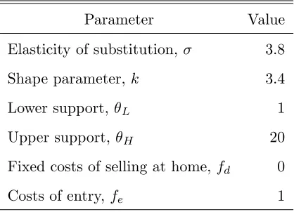
Note that a number of parameters in(17), namelyffe; fd; ; k; L; Hg, are not identi…able from
the trade data (i.e., the …t of the data does not vary as you change them). Therefore, I …x these
parameters at values consistent with other work.
In …xing , I follow the results in the previous studies estimating the elasticity of substitution.
Bernard et al. (2003) argue that equal to 3:8 captures the export behavior of the U.S.
plants best. Broda and Weinstein (2006) estimate the elasticity of substitution for di¤erent
aggregation levels. In period 1990-2001 for SITC-3 aggregation level, the estimates vary from
1:2 (thermionic, cold cathode, photocathode valves, etc.) to 22:1 (crude oil from petroleum or
bituminous minerals) with the mean equal to4. The number obtained in Bernard et al. (2003)
is close to the mean of the estimates in Broda and Weinstein (2006). Following their results, I
set equal to3:8.
The distribution of productivity draws in(15)is characterized by parameters L, H, andk.
I normalize Lto unity. In many studies, to simplify analytical derivations H is set to in…nity.22
However, setting H to in…nity implies that there always exist some relatively productive …rms
…nding it pro…table to export to any country. This means that the model will not generate
Table 1: The Values Assigned to the Unidenti…able Parameters
Parameter Value
Elasticity of substitution, 3:8
Shape parameter, k 3:4
Lower support, L 1
Upper support, H 20
Fixed costs of selling at home, fd 0
Costs of entry, fe 1
export zeros, which is at odds with the data. In the paper, I set H equal to 20. On the one
hand, …nite H allows for zero bilateral ‡ows. On the other hand, there is not much di¤erence in
terms of the statistics of the productivity distribution (such as average, variance, etc.) between
H = 20 and H =1. That is, the choice of H is mainly consistent with the previous studies
and allows for export zeros. The shape parameter k determines the behavior of the tail of the
…rm-speci…c productivity distribution. Following Ghironi and Melitz (2004) and Bernard et al.
(2007), I set kequal to3:4.
Following Helpman et al. (2008), I set fd equal to zero so that there are no …xed costs of
selling domestically, implying that all entering …rms serve the home market. Finally, as changes
in the parameter fe only rescale the mass of entrants into the industry and have no impact on
trade volumes, I normalizefe to unity.23
Hereafter, I assume that the set of parameters ffe; fd; ; k; L; Hg is …xed at the values
reported in Table 1. In Appendix B, I do several robustness checks by trying some other parameter values. I …nd that changes in the values do not substantially alter the quantitative
implications of the model.
4.2 Estimation Procedure
The rest of the parameters is given by = f 0; 1; 2; 3; 4; 5; fx; g. To estimate these
parameters, I use a restricted non-linear least squares procedure. For given andfZi; Ligi=1::N,
we can solve the system of equations (12)and …nd the equilibrium values offwi,Pi,Meigi=1::N
2 3The condition(28)implies that any changes inf
ij andfeikeeping fij
fei …xed for alljdo not a¤ect the cuto¤s
(notice that if we know , we can constructf ijgi;j=1::N using (16)). Let Xij(Z; L; ) denote
the value of exports from countryitojgenerated by the model conditional on ,fZi; Ligi=1::N,
and the corresponding equilibrium values of fwi, Pi, Meigi=1::N (here Z = fZigi=1::N and
L=fLigi=1::N). In words, if we know the parameters of the model and the exogenous variables
Z and L, we can solve for the equilibrium and construct the corresponding bilateral trade ‡ows.
To estimate , I solve the following minimization problem:
minPi;j:i6=j Xijo Xij(Z; L; ) 2 (18)
subject to
(Z; L; ) = 0, (19)
where Xijo is the value of exports from i to j observed in the data. (Z; L; ) stands for the di¤erence between the number of zeros predicted by the model (given andfZi; Ligi=1::N) and
the actual number of zero bilateral trade ‡ows in the data (the "actual" zeros).24 This estimation
technique also allows to account for the general equilibrium features of the model (including the
e¤ects of free entry into the industry) and to use the information contained in export zeros. The
restriction(19)is imposed for identi…cation purposes. In particular, the variable and …xed costs
of trade are not separately identi…able from just bilateral trade data. Any changes in fx can be
o¤set by proper changes in f 0; 1; 2; 3; 4; 5; gwithout a¤ecting the value of the objective
function in(18).
The estimation procedure discussed above is based on the fact that we know the values of
fZi; Ligi=1::N. While for fLigi=1::N we can use the data on population size in the countries,
2 4The estimation procedure implies that the model …ts just the number of zeros. However, it is possible that
the model generates zeros that are not actually observed in the data and vice versa. Therefore, we can decompose
(Z; L; )into the sum of two terms:
(Z; L; ) = T(Z; L; ) + F(Z; L; ): (20)
In (20), T(Z; L; ) is the di¤erence between the number of correctly predicted zeros (zeros predicted by the
model and observed in the data) and the number of "actual" zeros, while F(Z; L; ) is the mismatch (zeros
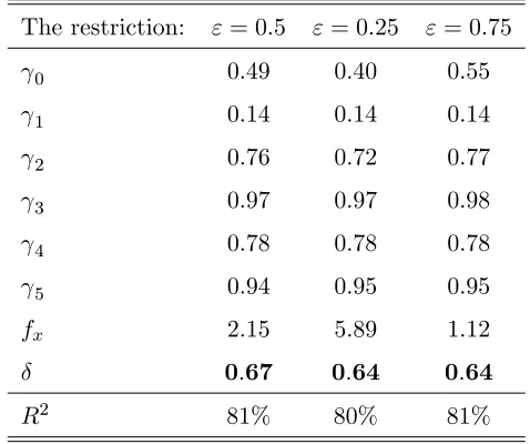
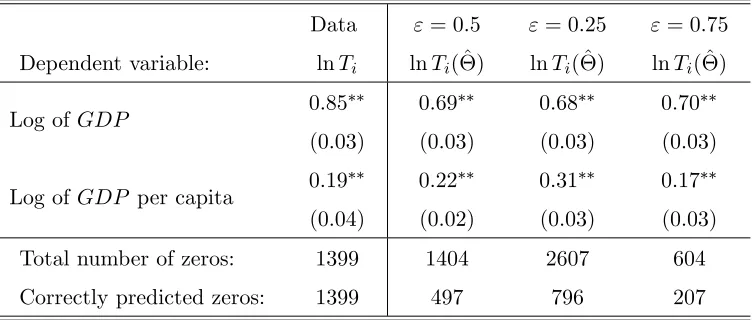
that are predicted by the model but not observed in the data). Hence, the restriction (19)implies that equal weights are attached to T(Z; L; )and F(Z; L; ). In AppendixC, I examine alternative restrictions in the
minimization problem. In particular, I consider the following restriction:
(1 ") T(Z; L; ) +" F(Z; L; ) = 0,
fZigi=1::N are not observable. To resolve this problem, I use the data on per capita income
levels to reconstruct fZigi=1::N. Speci…cally, from the equilibrium conditions(12) we have that
w=w(Z; L; ), wherew=fwigi=1::N. This implies that we can expressZin terms ofw,L, and
the parameters . That is, we can invert the function w(Z; L; ) and obtainZ =Z(w; L; ).25
In the model,wiis equal to per capita income in countryi, which is observed in the data. Hence,
using the data for fwigi=1::N we can reconstruct fZigi=1::N. In this case, the minimization
problem can be rewritten as follows:
minPi;j:i6=j Xijo Xij(Z(w; L; ); L; )
2
(21)
subject to
(Z(w; L; ); L; ) = 0. (22)
Note that the structure of the equations in (12) is nonlinear. This implies that the function
w(Z; L; ) is not necessarily one-to-one. For instance, several di¤erent values ofZ may lead to
the same value of w. However, no such examples occur in the numerical analysis I conduct in
the paper.
Notice that in the model,Li can be interpreted not only as population size in countryi, but
also as the size of labor force in that country. In the paper, I use the data on population sizes
to constructfLigi=1::N, while I also estimate the model using the data on the size of labor force
in the countries. I …nd that the results do not substantially di¤er from those obtained in the
paper.
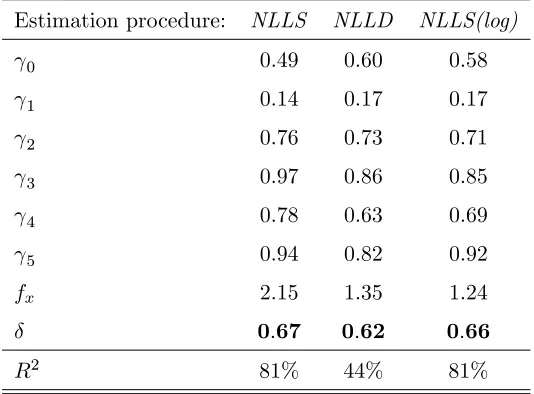
In Appendix D, as a robustness check I consider alternative estimation procedures such as
non-linear least deviations and non-linear least squares applied to logarithms rather than levels.
I …nd that these estimation procedures yield similar predictions as the procedure used in the
paper.
4.3 Results
As a measure of the explanatory power of the model, I use
R2 = 1
P
i;j:i6=j Xijo Xij(Z(w; L; ); L; )
2
P
i;j:i6=j Xijo
2 .
The explanatory power is 100%, if we are able to …t perfectly all bilateral trade ‡ows: i.e.,
P
i;j:i6=j Xijo Xij(Z(w; L; ); L; )
2
= 0.
2 5Z
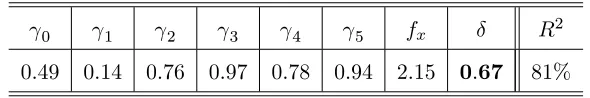
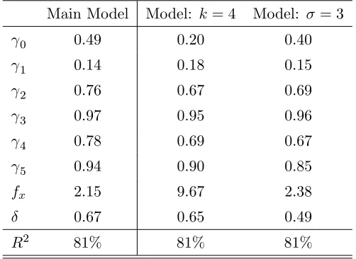
Table 2 reports the results obtained from solving (21) subject to (22).26 The explanatory power of the model is 81%. Like in traditional estimates of the gravity equation, the results
show that country iand j trade more if they are closer to each other, have a common border,
share a common language, or belong to the same regional trade agreement (NAFTA or EU). The
estimated value of is 0:67, implying a strong correlation between country development level
and market access costs. More developed countries tend to have lower …xed costs of exporting
relative to the other costs.
To compare the quantitative implications of the model with the data, I run the following
regression (robust standard errors in parentheses):
ln Ti
Ti( ^ )
= 1:23
(0:09) + 0
:16
(0:03)lnGDPi (00::0404)ln
GDPi
Li
, (23)
whereTi is the actual trade volumes of countryiandTi( ^ ) is the volumes of trade generated by
the model given the estimated values of the parameters (seeTable 2). As we can see from(23), the model captures the e¤ect of per capita income on trade volumes (conditional on total income)
quite well. The corresponding coe¢cient is not signi…cantly di¤erent from zero. Meanwhile,
the estimates in (23) suggest that the model somewhat underestimates trade volumes of large
population countries. Table 3 reports the elasticities of trade with respect to total and per capita incomes observed in the data and generated by the model (the …rst and second columns,
respectively). In the data, doubling a country income per capita (keeping the total income
unaltered) leads on average to an increase in trade volumes of 19% and doubling a country
population size raises trade volumes by85%. The model predicts a rise in trade volumes of22%
and 69%, respectively.
Recall that the restriction (22) in the estimation procedure implies that the number of
zero bilateral trade ‡ows generated by the model is the same as that in the data. As it was
discussed above, mismatch is possible. I …nd that the model explains 35% of the zeros in the
data. That is, 35%of zeros generated by the model match the zeros observed in the data, while
the rest is mismatch. The key point is that the model underestimates trade volumes of large
population countries. As a result, it generates a number of "false" zeros among countries with
large population and does not predict many zeros in the data among small population countries.
Notice that the estimated association between a country development level and …xed costs of
trade helps to explain many zeros in the data. In the next subsection, I estimate a variation of
2 6I do not report the asymptotic errors, as it is extremely hard to explore the asymptotic properties of the
Table 2: Parameter Estimates
0 1 2 3 4 5 fx R2
0:49 0:14 0:76 0:97 0:78 0:94 2:15 0:67 81%
the model when is equal to zero: i.e., …xed costs of trade (in terms of labor units) are identical
across the countries. I …nd that in this case, the mismatch constitutes 91%.
The estimated values of the parameters also allow us to determine the magnitude of …xed
costs of trade. For each country I construct the ratio of the aggregate …xed costs of exporting
to the aggregate export pro…ts, which is given by
F CRi=
MeiPNj6=i(1 G( ij))fij
MeiPNj6=i
R H
ij ij( )dG( )
.
The ratios vary from 0:32 (for Iceland) to0:64 (for India) with the mean equal to 0:45. That
is, the total costs of access to foreign markets constitute on average around the half of the total
export pro…ts. The similar result is obtained in Eaton et al. (2008), who …nd that the share of
…xed costs in the gross pro…ts is a little more than half. By regressing the log of F CRi on the
logs ofGDP andGDP per capita, I …nd that richer countries have the lower share of …xed costs
of exporting in the total export pro…ts, while countries with larger population have the higher
share. Namely,
lnF CRi = 0:84
(0:01)
+ 0:04
(0:003)lnGDPi (00::002)14 ln
GDPi
Li
. (24)
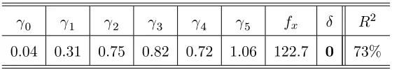
In the next subsection, I estimate the model when is equal to zero and compare the
quantitative implications of that model with those obtained above.
4.3.1 Identical Market Access Costs: Comparison
If is equal to zero, then
fij =wifx for i6=j,
implying identical …xed costs of trade (in terms of labor) across countries. Since I …x at zero,
the set of parameters estimated isf 0; 1; 2; 3; 4; 5; fxg.
Table 4reports the estimated values of the parameters. The explanatory power of the model falls from81%to73%. Hence, di¤erences in …xed costs of trade established in the model explain
Table 3: Trade Elasticities and Zeros
Estimator:
Dependent variable:
Data (OLS)
lnTi
Model (OLS, >0)
lnTi( ^ )
Model (OLS, = 0)
lnTi( ^ )
Log of GDP 0:85
(0:03)
0:69
(0:03)
0:76
(0:03)
Log of GDP per capita 0:19
(0:04)
0:22
(0:02)
0:04
(0:02)
Correctly predicted zeros: 100% 35% 9%
Observations: 100 100 100
Table 4: Parameter Estimates ( =0)
0 1 2 3 4 5 fx R2
0:04 0:31 0:75 0:82 0:72 1:06 122:7 0 73%
elasticities generated by the model with equal to zero. As it can be seen from the table, the
model does slightly better in predicting trade volumes of large population countries. Doubling
a country population size raises trade volumes by 76% compared to an increase of 85% in the
data. However, the e¤ect of per capita income on trade volumes is signi…cantly lower than that
in the data. Conditional on the total income, doubling a country income per capita leads on
average to an increase in trade volumes of 4%, while the e¤ect observed in the data is 19%.27
Finally, the percentage of correctly predicted zeros is 9%. This constitutes the mismatch of
91%, which is substantially greater than the mismatch obtained in the case when …xed costs of
exporting depend on a country development level.
2 7The positive and signi…cant (at the5%signi…cance level) e¤ect of per capita income on trade volumes in the
[image:21.612.173.458.321.371.2]5
Eliminating Asymmetries in Trade Costs
In this section, I use the estimated model to explore how the elimination of asymmetries in …xed
costs of trade a¤ects consumer welfare across countries. Speci…cally, I consider an experiment
where falls from0:67(the estimated value of ) to zero and examine the corresponding changes
in consumer welfare. Remember that setting to zero removes the relationship between market
access costs and development levels and, therefore, leads to symmetric …xed costs of trade:
fij =wifx for i6= j. The other parameters including Z are …xed at the values obtained from
the benchmark estimation procedure (seeTable 2).
Consumer welfare in country i (denoted as Wi) is equal to the real wage in that country.
Namely, fori= 1::N
Wi
Qi
Li
= wi
Pi
: (25)
Hence, given the parameters of the model, we can solve (12) for fwi; Pi; Meigi=1::N and then
using (25), …nd the equilibrium value of consumer welfare in country i. Let us denote 4Wi
Wi as
the percentage change in welfare in countryigiven the changes in the parameters of the model.
That is,
4Wi
Wi
= W
af ter i
Wibef ore 1,
where Wibef ore is the equilibrium value of welfare when the parameters are equal to their esti-mated values and Wiaf ter is welfare when is equal to zero (recall that the other parameters remain unchanged).
I …nd that all countries gain from the elimination of asymmetries in market access costs with
the average percentage change in welfare being equal to 17%. The next regression illustrates
how the gains depend on country characteristics. In particular, I regress 4Wi
Wi on the logs of
GDPi and GDPLi i:
4Wi
Wi
= 0:35
(0:01) (00::005)03 lnGDPi (00::005)05 ln
GDPi
Li
. (26)
As it can be seen, doubling a country population size on average reduces the welfare gains
by 3%, while doubling a country per capita income (controlling for the total income of that
country) reduces the gains by 5%. The former e¤ect is explained by the fact that setting to
zero enhances trade in all countries. Since countries with larger population tend to have a lower
trade to GDP ratio, those countries gain less compared to small population countries. The
development level: i.e., …rms in less developed countries face higher market access costs. Since
…xing at zero eliminates this relationship, the changes in welfare are more substantial for less
developed countries. I also …nd that removing asymmetries in …xed costs of trade dramatically
reduces the number of zero bilateral trade ‡ows. In the new equilibrium (after setting to zero),
there are only4 export zeros in comparison with 1399zeros when is equal to 0:67.
The …ndings above suggest that eliminating asymmetries in …xed costs of trade not only
raises consumer welfare, but also reduces welfare inequality across countries (as poor countries
gain relatively more). In particular, as a measure of the welfare inequality in the model, I
consider the ratio of the average income of the ten richest (in real terms) countries to that of
the ten poorest countries. I …nd that setting to zero reduces the measured welfare inequality
by 28%.
6
Alternative Speci…cations
In this section, I consider two alternative speci…cations of the model. First, I assume that …xed
costs of trade depend on both exporter’s and importer’s development levels. Second, I examine
the case when variable costs of trade depend on exporter’s development level, while …xed costs
of trade are identical across countries.
In the paper, …xed costs of trade depend only on characteristics of an exporting country.
Meanwhile, Arkolakis (2008) emphasizes that to serve a foreign market …rms may need labor
services from both the source and the destination countries. Eaton et al. (2008) assume that
market access costs depend only on importer characteristics. To account for the importer e¤ect
on …xed costs, I assume that
fij =
wi
Zi Zjfx fori6=j.
That is, …xed costs of exporting depend on importer’s development level as well. I then estimate
the model applying the same estimation procedure as before. The set of the parameters I
estimate is given by f 0; 1; 2; 3; 4; 5; fx; ; g.
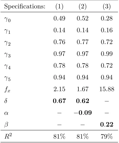
The second column in Table 5 shows the estimates of the parameters (the …rst column reports the estimates obtained in the benchmark case). As it can be inferred, there is a negative
correlation between the importer development level and the …xed costs of trade. The estimate of
is 0:09 implying that it is relatively easier to export to more developed countries. However,
Table 5: Alternative Speci…cations: Parameter Estimates
Speci…cations: (1) (2) (3)
0 0:49 0:52 0:28
1 0:14 0:14 0:16
2 0:76 0:77 0:72
3 0:97 0:97 0:99
4 0:78 0:78 0:72
5 0:94 0:94 0:94
fx 2:15 1:67 15:88
0:67 0:62
0:09
0:22
R2 81% 81% 79%
of the exporter development level. The presence of the importer e¤ect does not considerably
a¤ect the estimates of the other parameters and does not improve the explanatory power of the
model. This suggests that the importer e¤ect does not contribute a lot in explaining the bilateral
trade ‡ows. The third column in Table 6 reports the trade elasticities and the percentage of zeros correctly predicted by the model. As it can be seen, the presence of the importer e¤ect
does not signi…cantly change the trade elasticities and slightly improves the ability of the model
to match zeros in the data.
In his paper, Waugh (2009) assumes that variable trade costs are a function of symmetric
relationships and an exporter …xed e¤ect. He …nds a negative correlation between exporter per
capita income and the …xed e¤ect, implying that poor countries face higher variable trade costs
than rich countries. Following Waugh (2009), I examine a variation of the model when …xed
costs of trade are identical across countries, while variable trade costs depend on the exporter
development level. That is, for i6=j
fij = wifx and
ij = 1 + 0
Zi D
1
ij Bij
2
LN Gij
3
N AFij
4
EUij
5 .
Table 6: Alternative Speci…cations: Trade Elasticities and Zeros
Dependent variable:
Data
lnTi
(1)
lnTi( ^ )
(2)
lnTi( ^ )
(3)
lnTi( ^ )
Log ofGDP 0:85
(0:03)
0:69
(0:03)
0:69
(0:03)
0:68
(0:03)
Log ofGDP per capita 0:19
(0:04)
0:22
(0:02)
0:24
(0:03)
0:49
(0:03)
Correctly predicted zeros: 100% 35% 36% 27%
Observations: 100 100 100 100
lower variable costs of trade. I then estimate the parametersf 0; 1; 2; 3; 4; 5; fx; g.
The third column in Table 5 reports the parameter estimates. The estimate of is 0:22
meaning a strong negative correlation between variable costs of trade and country development
levels, which is consistent with the …ndings in Waugh (2009). The explanatory power slightly
falls from 81% to 79%. However, this variation of the model considerably overestimates the
impact of per capita income on trade volumes (see the fourth column in Table 6). The model predicts that controlling for the total income, doubling a country income per increases trade
volumes of that country by 49% (compared to 19% in the data). Moreover, the percentage
of correctly predicted zeros falls from 35% to27% constituting larger mismatch between zeros
predicted by the model and those in the data.
Hence, while the relationship between variable costs of trade and development levels can also
account for greater trade volumes of richer countries and zero trade ‡ows in the data, the model
in this case performs much worse in matching the trade elasticities and zeros in the data.
7
Concluding Remarks
This paper contributes to a rapidly growing literature analyzing the role of …xed costs of trade in
explaining trade volumes. I show that an association between …xed costs of trade and countries’
development levels can qualitatively and quantitatively account for the relationship between per
capita income and trade volumes observed in the data and explain a number of zeros in bilateral
There are several directions in which further research can be pursued. First, in the paper, the
association between market access costs and development levels is estimated to match the data
on aggregate trade volumes. It might seem desirable, however, to estimate this association using
micro-level ("independent") data and then to examine how much of the relationship between per
capita income and trade volumes is explained by the variation in …xed costs of trade. Secondly, it
might be interesting to incorporate nonhomothetic preferences in the model. This would enable
us to capture the e¤ects of both consumer preferences and market access costs on trade volumes
in a general equilibrium framework. Finally, in the paper, I consider an environment where
countries trade only in a di¤erentiated good. This framework is more applicable to the case of
trade among rich countries. In particular, the setup of the model assumes away the possibility
that trade ‡ows can be generated by di¤erences in factor endowments. To explain better trade
between countries with di¤erent factor endowments, we can extend the model by incorporating
the Heckscher-Ohlin trade theory (see for example Bernard et al. (2007)). This would allow us
to analyze both intra-industry and inter-industry trade and, thereby, to improve the …t of the
References
Arkolakis, C. (2008), "Market Penetration Costs and the New Consumers Margin in
Interna-tional Trade," NBER WP 14214.
Bernard, A. B., Eaton, J., Jensen, J. B. and Kortum, S. (2003), "Plants and Productivity in
International Trade," American Economic Review, 93(4), 1268-1290.
Bernard, A. B., Redding, S. and Schott, P. K. (2007), "Comparative Advantage and
Heteroge-neous Firms," Review of Economic Studies, 74(1), 31-66.
Broda, C. and Weinstein, D. E. (2006), "Globalization and the Gains from Variety," Quarterly
Journal of Economics, 121(2), 541-585.
Centre d’Etudes Prospectives et d’Informations Internationales, CEPII (2005), The CEPII
Databases-Distances, http://www.cepii.fr/anglaisgraph/bdd/distances.htm
Chaney, T. (2008), "Distorted gravity: the Intensive and Extensive Margins of International
Trade," American Economic Review, 98(4), 1707-1721.
Chen, M., Otsuki, T. and Wilson, J. (2006), "Do Standards Matter for Export Success?" World
Bank Policy Research Working Papers. No. 3809.
Doing Business (2006), "Doing Business 2006," The World Bank Group,
http://www.doingbusiness.org
Eaton, J. and Kortum, S. (2002), "Technology, Geography, and Trade." Econometrica, 70(5),
1741-79.
Eaton, J., Kortum, S. and Kramarz F. (2008), "An Anatomy of International Trade: Evidence
from French Firms," University of Minnesota, mimeograph.
Feenstra, R., Lipsey, R. E., Deng, H., Ma, A. C. and Mo, H. (2005), "World Trade Flows:
1962-2000," NBER Working Paper, No. 11040.
Fieler, A. C. (2009), "Non-Homotheticity and Bilateral Trade: Evidence and a Quantitative
Explanation," working paper.
Flam, H. and Helpman, E. (1987), "Vertical Product Di¤erentiation and North-South Trade,"
Ghironi, F. and Melitz, M. (2005), "International Trade and Macroeconomic Dynamics with
Heterogeneous Firms," Quarterly Journal of Economics, 120(3), 865-915.
Helpman, E., Melitz, M. and Rubinstein, Y. (2008), "Estimating Trade Flows: Trading Partners
and Trading Volumes," Quarterly Journal of Economics, 123(2), 441-487.
Hummels, D. and Klenow, P. J. (2002), "The Variety and Quality of a Nation’s Trade," NBER
WP 8712.
Hunter, L. C. (1991), "The Contribution of Nonhomothetic Preferences to Trade," Journal of
International Economics, 30, 345–58.
Johnson, R. C. (2007), "Trade and Prices with Heterogeneous Firms," UC Berkeley,
mimeo-graph.
Markusen, J. (1986), "Explaining the Volume of Trade: An Eclectic Approach," American
Economic Review, 76, 1002–1011.
Matsuyama, K. (2000), "A Ricardian Model with a Continuum of Goods under Nonhomothetic
Preferences: Demand Complementarities, Income Distribution, and North-South Trade,"
Jour-nal of Political Economy, 108, 1093-1120.
Melitz, M. (2003), "The impact of trade on intraindustry reallocations and aggregate industry
productivity," Econometrica, 71(6), 1695-1725.
Mersha, T. (1997), "TQM Implementation in LDCs: Driving and Restraining Forces,"
Interna-tional Journal of Operations and Production Management, 17(2), 164-183.
Mitra, D. and Trindade, V. (2005), "Inequality and Trade," Canadian Journal of Economics,
38, 1253-1271.
Nordas, H., Pinali, E. and Gross, MG. (2006), "Logistics and Time as a Trade Barrier," OECD
Trade Policy Working Papers, No 35.
Potoski, M. and Prakash, A. (2009), "Information Asymmetries as Trade Barriers: ISO 9000
Increases International Commerce," Journal of Policy Analysis and Management, 28(2), 221-238.
Stokey, N. (1991), "The Volume and Composition of Trade between Rich and Poor Countries,"
United Nation Statistics Division (2007), "Industrial Statistics Database," 2007,
http://comtrade.un.org/db/default.aspx
Waugh, M. (2009), "International Trade and Income Di¤erences," University of Iowa,
mimeo-graph.
Appendix
A
: Per Capita Income and Trade Volumes
In this section, I prove Proposition 1. The outline of the proof is as follows (see the details of the proof in the subsections). Suppose that country 2 trades more in the equilibrium. Since
trade is balanced, country2 imports more than country 1. That is,
PN
j>2Xj2 PNj>2Xj1. (27) As total incomes in the countries are the same (w1L1 =w2L2), (27) immediately implies that
the price index in country 2 is higher than that in country 1: P2 P1. Next, I show that if
P2 P1 and the assumptions of the proposition hold, then country1exports more than country
2. This constitutes a contradiction, implying that country 1 trades strictly more than country
2 in the equilibrium. This stage of the proof has two steps.
Step 1: The free entry condition in (12)states that
fei=
N
X
j=1
Pr ( ij)E(( ij( ) fij)j ij).
Using the expression for ij( )in (6)and dividing ij( )by ij( ij), we obtain that
ij( ) ij( ij)
=
ij
1
()
ij( ) = ij( ij) ij
1 .
Taking into account that ij( ij) =fij, the free entry condition for country ican be rewritten
as follows: N X j=1 fij fei Z H ij ij 1 1 !
dG( ) = 1. (28)
Hence, condition (28) implies that for countries 1 and 2 (recall that countries 1 and 2 do not
trade with each other):
N
X
j:j6=2
f1j
fe1
Z H
1j 1j
1
1 !
dG( ) =
N
X
j:j6=1
f2j
fe2
Z H
2j 2j
1
1 !
dG( ). (29)
Note that f1j
fe1 is strictly less than or equal to
f2j
fe2 for all j= 1::N. This implies that at least for
somej,
Z H
1j 1j
1
1 !
dG( )>
Z H
2j 2j
1
1 !
Otherwise, (29) does not hold. This implies that 1j < 2j for some j. I show that in fact,
1j < 2j for all j > 2 (see details in the next subsection). That is, country 1 has a higher
fraction of …rms in the total mass of entrants exporting to country j for any j >2.
Step 2: Next, I show that country 1has higher exports to domestic sales ratio than country
2. This means that country 1 exports more than country 2, as total incomes of the countries
are the same. In the next subsection, I show that the result of the previous step and the fact
that f1j
f11 is strictly less than
f2j
f22 for all j >2 imply that R H
1j
1dG( )
R H
11
1dG( ) >
R H
2j
1dG( )
R H
22
1dG( ) for all j >2. (30)
As we assume that 1j = 2j for allj >2,(30) implies that
PN j>2 11j
1 w
jLj
Pj1
R H
1j
1dG( )
R H
11
1dG( ) >
PN j>2 12j
1 w
jLj
Pj1
R H
2j
1dG( )
R H
22
1dG( ) .
Note thatP2 P1 implies that Pw11L1 1
w2L2
P21 . This in turn means that
PN j>2 11j
1 w
jLj
Pj1
R H
1j
1dG( )
w1L1
P11
R H
11
1dG( ) >
PN j>2 12j
1 w
jLj
Pj1
R H
2j
1dG( )
w2L2
P21
R H
22
1dG( ) ,
which is equivalent to
PN j>2X1j
X11
>
PN j>2X2j
X22
.
This …nishes the proof. In the next sections, I provide the details of the proof.
Proof of Step 1
At this stage of the proof, I show that 1j < 2j for all j > 2. Speci…cally, I …rst show that if
1j < 2j for some j >2, then 1j < 2j for all j >2. Then, I prove that the equality (29)
implies that 1j < 2j at least for somej >2. This …nishes the proof.
From the zero pro…t condition(7),
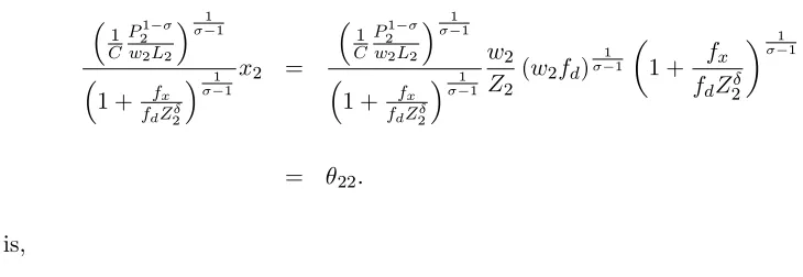
ij = wi Zi ij 1 C Pj1 wjLj
Substituting for fij, the cuto¤s are given by
11 =
w1
Z1
(w1fd)
1 1 1
C P11 w1L1
1 1 ; (31) 22 = w2 Z2
(w2fd)
1 1 1
C P21 w2L2
1 1 ; (32) ij = wi Zi
(wifd)
1
1 1 + fx
fdZi
1 1
ij
1
C Pj1 wjLj
! 1 1
forj >2 andi= 1;2. (33)
Given the expressions for the cuto¤s, it is straightforward to show that if 1j < 2j for some
j >2, then
w1
Z1
(w1fd)
1
1 1 + fx
fdZ1
1 1
1j
1
C Pj1 wjLj
! 1 1
< w2
Z2
(w2fd)
1
1 1 + fx
fdZ2
1 1
2j
1
C Pj1 wjLj
! 1 1
.
As we assume that 1j = 2j for allj >2, the last inequality implies that
w1
Z1
(w1fd)
1
1 1 + fx
fdZ1
1 1
< w2 Z2
(w2fd)
1
1 1 + fx
fdZ2
1 1
.
This in turn means that 1j < 2j for all j >2.
To reduce the notation in this subsection, I denote R H ij ij
1
1 dG( ) as H( ij).
Notice that H0( ij)<0. Given the new notation, the equality (29) can be rewritten as follows
(recall that country 1and 2 do not trade with each other):
N
X
j>2
f1j
fe1
H( 1j) +
f11
fe1
H( 11) =
N
X
j>2
f2j
fe2
H( 2j) +
f22
fe2
H( 22).
Substituting for fe1,fe2,f1j,f2j,f11, and f22 (see (11)and (10)), we have
fd
fe
+ fx
Z1
N
X
j>2
H( 1j) +
fd
fe
H( 11) =
fd
fe
+ fx
Z2
N
X
j>2
H( 2j) +
fd
fe
H( 22). (34)
To …nish the proof, I consider w1
Z1w 1
1
1 and wZ22w 1
1
2 . In general, we do not know whether
w1
Z1w 1
1
1 is greater or less than wZ22w 1
1
2 in the equilibrium. Therefore, we need to examine two
cases. First, if w1
Z1w 1
1
1 < wZ22w 1
1
2 , then (asZ1 > Z2),
w1
Z1
(w1fd)
1
1 1 + fx
fdZ1
1 1
< w2 Z2
(w2fd)
1
1 1 + fx
fdZ2
1 1